TITLE: Scraping plot locations from the ForestPlots.net web map
DATE: 2023-10-05
AUTHOR: John L. Godlee
====================================================================
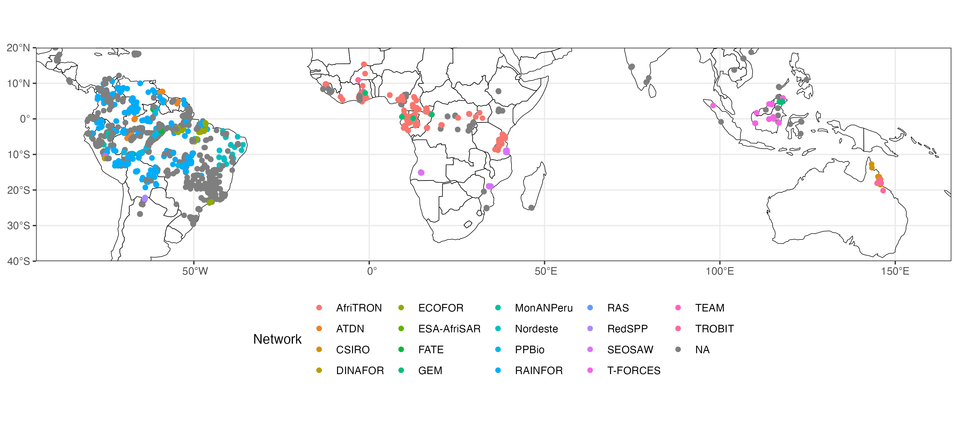
I was making a presentation about vegetation monitoring networks
and wanted a map showing the spatial distribution of vegetation
monitoring plots across the tropics. ForestPlots.net is a
meta-network which holds a database of plot-based tree demographic
data. They have a web map with useful metadata, but this map
doesn't look great and I didn't want to just include a screenshot.
[ForestPlots.net]:
https://forestplots.net/
[web map]:
https://forestplots.net/en/map
Looking at the source for the webpage, I saw that the map is
embedded, with this URL:
https://georgeflex.maps.arcgis.com/apps/Embed/index.html?webmap=df5f
3c6ca21a44c5ba7c39d9355ff9dd&extent=-108.9111,-61.228,76.7139,43.516
7&zoom=true&previewImage=false&scale=true&disable_scroll=true&theme=
light
The ID of the map is an API endpoint that can be used to load the
data underlying the map directly:
https://www.arcgis.com/sharing/rest/content/items/df5f3c6ca21a44c5ba
7c39d9355ff9dd/data
From there, I can save the JSON file and process it further in R.
First I load some packages and import the data:
# Packages
library(rjson)
library(dplyr)
library(sf)
library(rnaturalearth)
library(ggplot2)
# Import data
json_file <- "./fp_arcgis_fmt.json"
dat <- fromJSON(paste(readLines(json_file), collapse = ""))
Then I need to extract the map features from the JSON file. It took
some trial and error to understand the structure of the JSON:
# Extract feature collections from JSON file
f <-
lapply(dat$operationalLayers[2:length(dat$operationalLayers)],
function(x) {
x$featureCollection$layers[[1]]$featureSet$features
})
# Combine the feature collections into one list
fu <- unlist(f, recursive = FALSE)
# Extract metadata and plot locations
fl <- lapply(fu, function(x) {
list(
lon = as.numeric(x$geometry$x),
lat = as.numeric(x$geometry$y),
plot_id = as.character(x$attributes$PlotCode),
country = as.character(x$attributes$Country),
plot_type = as.character(x$attributes$plottype),
network = as.character(x$attributes$Network),
prinv = as.character(x$attributes$PI_map))
})
# Replace NULL entries with NA
flc <- lapply(fl, function(x) {
lapply(x, function(y) {
if (is.null(y) | length(y) == 0) {
NA_character_
} else {
y
}
})
})
# Make dataframe with metadata and plot locations
fdf <- bind_rows(lapply(flc, as.data.frame))
Then to create the map I need to convert the dataframe into an sf
object and transform the projection from web Mercator (3857) to
WGS84 (4326), get the world map object, and recode the network
names to make the legend easier to read:
# Make into sf dataframe
fsf <- st_as_sf(fdf, coords = c("lon", "lat"), crs = 3857) %>%
st_transform(4326)
# Get world map
world <- ne_countries(returnclass = "sf")
# Recode network names
fsf$network <- case_when(
fsf$network %in% c("AfriTRON", "AfriTRON / TROBIT") ~
"AfriTRON",
fsf$network == "." ~ NA_character_,
fsf$network %in% c("COL-TREE", "COL-TREE / RAINFOR",
"RAINFOR", "RAINFOR / COL-TREE") ~ "RAINFOR",
fsf$network %in% c("FATE", "FATE / RAINFOR", "FATE/CNPQ") ~
"FATE",
fsf$network %in% c("GEM", "GEM / TROBIT", "GEM/AfriTRON",
"SAFE GEM") ~ "GEM",
fsf$network == "TEAM / MonANPeru" ~ "TEAM",
TRUE ~ fsf$network)
Then finally I can create the map
# Create map
fp_map <- ggplot() +
geom_sf(data = world, fill = NA, colour = "black", size =
0.4) +
geom_sf(data = fsf, aes(colour = network)) +
scale_colour_discrete(name = "Network") +
theme_bw() +
theme(legend.position = "bottom") +
labs(x = NULL, y = NULL) +
coord_sf(expand = FALSE,
xlim = c(-95, 166),
ylim = c(-40, 20))
ggsave(fp_map, width = 11, height = 5, file = "fp_map.png")