TITLE: Shiny app to explore climate space of SEOSAW region
DATE: 2022-09-10
AUTHOR: John L. Godlee
====================================================================
I made an R Shiny web app to explore the climate space of the
SEOSAW region. The app can be found here, on shinyapps.io.
[here, on shinyapps.io]:
https://johngodlee.shinyapps.io/climate_space/
A big part of getting the app to run smoothly was to pre-process
the data sources so they could be loaded quickly from disk,
subsetted quickly, and rendered quickly with ggplot(). I haven't
styled the app much to make it look pretty, as it was more a
learning experience on how code reactive objects in Shiny.
I loaded country outlines of Africa and the SEOSAW ecoregion from
the {seosawr} R package, and simplified them using {rmapshaper}:
africa <- seosawr::africa
seosaw_region <- seosawr::seosaw_region
seosaw_bbox <- seosawr::seosaw_bbox
africa_simp <- ms_simplify(africa,
keep = 0.01, keep_shapes = FALSE) %>%
st_intersection(., seosaw_bbox)
seosaw_region_simp <- ms_simplify(seosaw_region,
keep = 0.01, keep_shapes = FALSE)
I used climate data from WorldClim, which I downloaded at 10 minute
spatial resolution using the {raster} package:
[WorldClim]:
https://www.worldclim.org/
bioclim <- getData("worldclim", var = "bio", res = 10)
which returns a raster stack object. Then I cropped and masked the
climate data with the SEOSAW region polygon:
bioclim_crop <- mask(crop(bioclim, seosaw_region_simp),
seosaw_region_simp)
and finally, extracted the values and coordinates of each raster
cell for each raster layer, resulting in a large matrix, with cells
for rows, and bioclim variables or coordinates as columns, which I
saved as a .rds file.
bioclim_val <- cbind(coordinates(bioclim_crop),
values(bioclim_crop))
bioclim_val_fil <- bioclim_val[
!apply(bioclim_val, 1, function(x) {
all(is.na(x[!names(x) %in% c("x", "y")]))
}),
]
saveRDS(bioclim_val_fil, "app/data/bioclim_val_fil.rds")
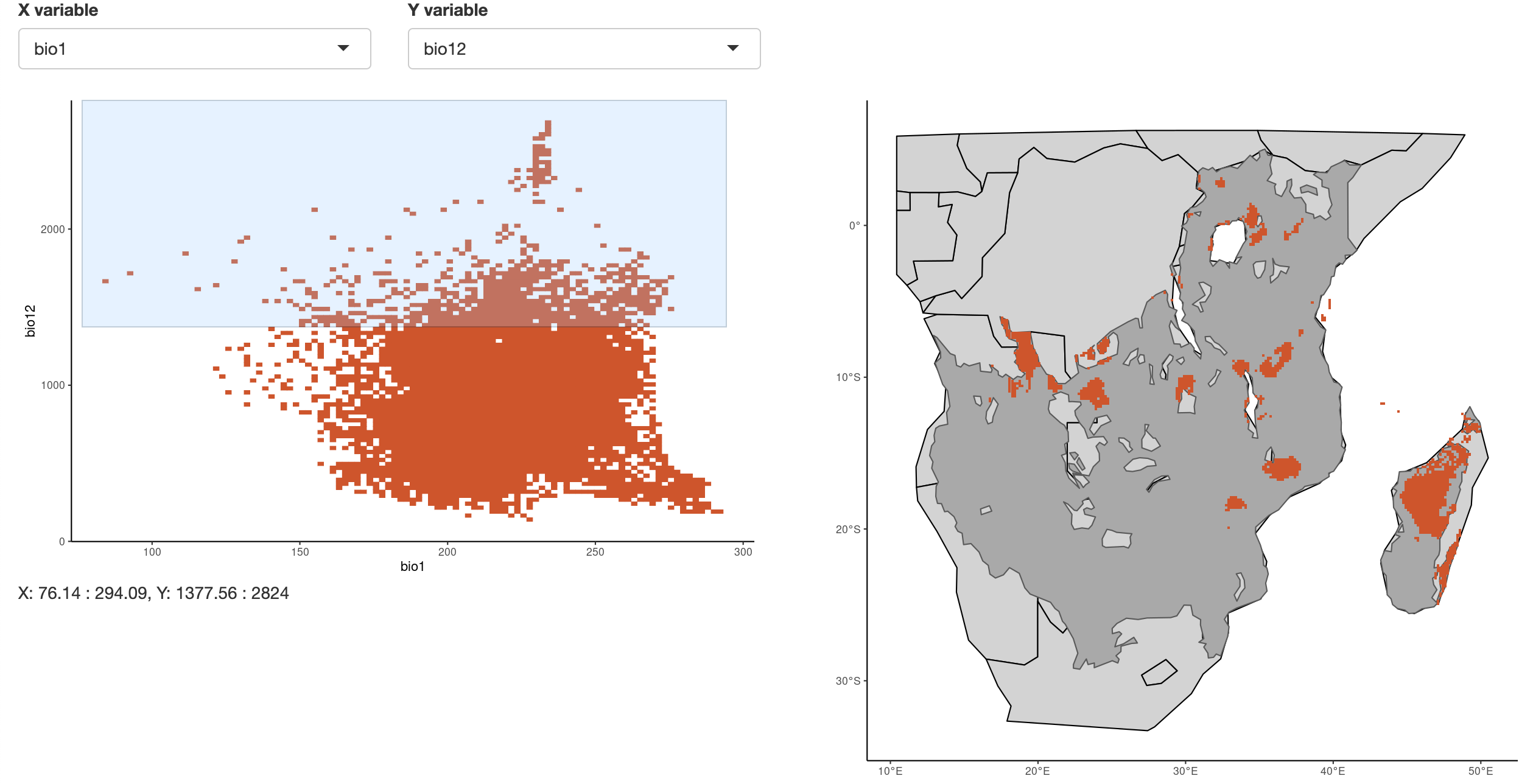
The app allows you to draw a rectangle around the climate space of
interest using two bioclim variables which you can select from a
dropdown list. This process uses the brush operator in the Shiny
plotOutput() function. I subsetted the raster matrix to the values
returned by input$brush using reactive() in the Shiny app.
rasterMapInput <- reactive({
val_sel <- val[,c("x", "y", input$xvar, input$yvar)]
if (!is.null(input$brush)) {
xmin <- input$brush$xmin
xmax <- input$brush$xmax
ymin <- input$brush$ymin
ymax <- input$brush$ymax
val_sel <- val_sel[
val_sel[,3] > xmin &
val_sel[,3] < xmax &
val_sel[,4] > ymin &
val_sel[,4] < ymax,
c("x", "y")]
}
as.data.frame(val_sel)
})
Then I simply used ggplot() with rasterMapInput() as the data input
to geom_tile() to map the climate space selected on the map of
southern Africa.
# Extract values from selected raster layers
valInput <- reactive({
as.data.frame(val[,c(input$xvar, input$yvar)])
})
output$plot1 <- renderPlot(
ggplot() +
geom_bin2d(data = valInput(),
mapping = aes_string(x = names(valInput())[1], y =
names(valInput())[2]),
colour = bg_col, fill = bg_col, bins = 100) +
theme_classic() +
theme(legend.position = "none")
)
output$plot2 <- renderPlot(
map_plot +
geom_tile(data = rasterMapInput(),
aes(x = x, y = y),
fill = bg_col)
)