TITLE: Comparing coordinates of tree stems collected with GPS or
tape measures
DATE: 2022-08-27
AUTHOR: John L. Godlee
====================================================================
In 2018 and 2019 I set up some 100x100 m (1 ha) permanent
vegetation monitoring plots in Bicuar National Park, southwest
Angola. We measured the stem diameter of each tree stem >5 cm
diameter and attached a numbered metal tag to each of these stems
so we could track the growth and mortality of each stem over time.
At the same time as measuring the stem diameters and attaching the
tags, I also took a quick GPS point with a Garmin GPSMAP 65s
Handheld GPS unit.
There are two main reasons to record the location of each stem in
the plot. The first is to make it easier to relocate stems in the
future. Sometimes tags fall off or stems are completely vaporised
by fire. If we know the location of the stem, we can visit that
location and confirm what has happened to the stem since the last
survey. The second reason is that if we understand the spatial
distribution of stems, we can better understand competitive (or
facilitative) interactions among individuals, and look at how these
interactions affect biomass dynamics.
When I revisited the plots in 2022, my goal was to collect lots of
auxiliary data, to enrich our picture of the ecosystem. Alongside
collecting data on woody debris, herbaceous biomass, and tree leaf
traits, I also recorded the position of stems that had recruited
since the initial survey back in 2018/2019. Instead of using a GPS,
this time I used tape measures to record the position of each stem,
using an XY coordinate system.
While we had the tape measures set up, I also re-recorded the
positions of existing stems so I could compare the two methods of
measuring the stem location. Others have encouraged me to use tape
measures, suggesting that the GPS isn't accurate enough, but tape
measures takes a long time in the field compared to a GPS. If the
accuracy of the GPS points is good enough, there's no need to waste
time with the tape measures.
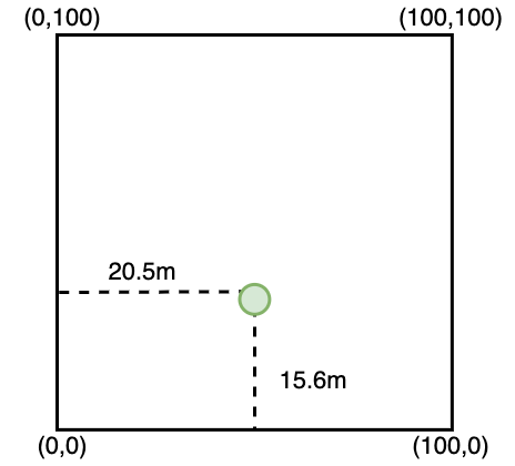
To make the latitude-longitude coordinates comparable with the XY
coordinates, I converted the lat-long coordinates to XY coordinates
using a function I wrote in R. Hopefully the comments on the code
suffice to describe what's going on, but the basic idea is that the
function takes a dataframe of stem measurements in multiple plots
and an {sf} polygons object with multiple plot polygons, linked by
the plot_id column. For each plot, the function follows this
process:
1. Find the southwest and southeast corners of the polygon
2. Rotate both the polygon and the stem locations so that the
SW-SE axis of the polygon runs exactly E-W.
3. Calculate the E-W and N-S distance from the southwest corner of
the plot to each stem location, in metres.
#' Convert lat-long stem coordinates to XY grid coordinates
#'
#' In rectangular plots to convert latitude and longitude
coordinates to XY
#' grid coordinates, using the southwest corner of the plot as
the origin point
#' (0,0), with the X axis increasing west -> east.
#'
#' @param x dataframe of stem data
#' @param polys sf object containing plot polygons, assumes all
are rectangular
#' @param stem_plot_id column name string of plot IDs in x
#' @param polys_plot_id column name string of plot IDs in polys
#' @param longitude column name string of stem longitude in x
#' @param latitude column name string of stem latitude in x
#' @param x_crs coordinate reference system (CRS) or EPSG code
of stem
#' coordinates.
#'
#' @return dataframe of measurement IDs with x_grid and y_grid
filled
#' with estimated XY grid coordinates. NA values returned
if
#' longitude and latitude were missing.
#'
#' @examples
#'
#'
#' @export
#'
gridCoordGen <- function(x, polys, stem_plot_id = "plot_id",
polys_plot_id = stem_plot_id, measurement_id =
"measurement_id",
longitude = "longitude", latitude = "latitude",
x_crs = 4326) {
# Split stems by plot_id
x_split <- split(x, x[[stem_plot_id]])
# For each plot
grid_all <- do.call(rbind, lapply(seq_along(x_split),
function(y) {
# Get plot ID
plot_id <- unique(x_split[[y]][[stem_plot_id]])
# Subset polys to plot ID
poly_fil <- polys[polys[[polys_plot_id]] == plot_id,]
# Convert corners to points
poly_points <-
as.data.frame(sf::st_coordinates(poly_fil)[1:4,1:2])
# Get UTM zone of corners
utm_string <- UTMProj4(latLong2UTM(mean(poly_points[,1]),
mean(poly_points[,2])))
# Convert polygons to UTM
poly_utm <- sf::st_transform(poly_fil, utm_string)
# Convert UTM polygons to points
points_utm <- sf::st_cast(poly_utm, "POINT", warn =
FALSE)[1:4,]
# Extract coordinates as dataframe
coords_utm <-
as.data.frame(sf::st_coordinates(points_utm)[1:4,1:2])
# Define points to match corners to
match_point <- sf::st_sfc(sf::st_point(
x = c(mean(coords_utm$X) - 1000, mean(coords_utm$Y) -
1000)))
other_point <- sf::st_sfc(sf::st_point(
x = c(mean(coords_utm$X) + 1000, mean(coords_utm$Y) -
1000)))
# Set CRS
sf::st_crs(other_point) <- utm_string
sf::st_crs(match_point) <- utm_string
# Get sw and se corner
sw_corner <- points_utm[sf::st_nearest_feature(match_point,
points_utm),]
se_corner <- points_utm[sf::st_nearest_feature(other_point,
points_utm),]
# Convert to WGS for geosphere compatibility
sw_wgs <- sf::st_coordinates(sf::st_transform(sw_corner,
4326))
se_wgs <- sf::st_coordinates(sf::st_transform(se_corner,
4326))
# Find rotation along SW,SE edge
xy_bearing <- geosphere::bearing(sw_wgs, se_wgs)
# Get centroid of polygon
cent <- sf::st_centroid(sf::st_geometry(poly_utm))
# Get location of sw corner
sw_cent <- sf::st_geometry(sw_corner)
# Convert angle to radians for rotation
angle <- NISTunits::NISTdegTOradian(90 - xy_bearing)
# Convert stem coords to sf object
x_sf <- st_as_sf(
x_split[[y]][,c(measurement_id, longitude, latitude)],
coords = c(longitude, latitude), na.fail = FALSE)
st_crs(x_sf) <- x_crs
# Transform stems sf to UTM
x_utm <- st_transform(x_sf, utm_string)
# Rotate the stems same as polygon
x_rot <- (sf::st_geometry(x_utm) - cent) * rot(angle) * 1 +
cent
sw_cent_rot <- (sw_cent - cent) * rot(angle) * 1 + cent
st_crs(sw_cent_rot) <- st_crs(points_utm)
st_crs(x_rot) <- st_crs(points_utm)
x_cent <- x_rot - sw_cent_rot
x_cent_df <- as.data.frame(st_coordinates(x_cent))
names(x_cent_df) <- c("x_grid", "y_grid")
# Add cordinates to dataframe
x_out <- cbind(st_drop_geometry(x_sf), x_cent_df)
# Sub in empty stems
if (any(!x_split[[y]][[measurement_id]] %in%
x_out[[measurement_id]])) {
missed_stems <- x_split[[y]][
!x_split[[y]][[measurement_id]] %in%
x_out[[measurement_id]],
c(measurement_id)]
x_out <- rbind(x_out, missed_stems)
# NaN to NA
x_out$x_grid <- fillNA(x_out$x_grid)
x_out$y_grid <- fillNA(x_out$y_grid)
}
# Return
x_out
}))
# Return
return(grid_all)
}
I then matched the measurements using the tag ID of each stem,
calculated the distance between them, and the angle between the
tape measure and the GPS using this function:
# Define function to calculate angle of line, in radians
calcAngle <- function(x, y) {
dst_diff <- as.numeric(x - y)
return(atan2(dst_diff[1], dst_diff[2]) + pi)
}
First, here is a map where I laid all the location errors from each
of the 11 plots on top of each other.

One really interesting thing about the plot above is that it looks
like the errors get larger in the top part of the plot, and also
that the errors on the X axis are larger than the errors on the Y
axis.
In the field we always started collecting the XY coordinates from
the SW (bottom-left) corner of the plot, doing 20 m lines of trees
running E-W up to the NE corner. I wonder if the errors are larger
at the top of the plot because we were getting tired towards the
end of the day. Or maybe they were due to tape measure stretch?
Also from this plot I get the impression that the errors are
generally larger on the E-W axis than on the N-S axis. I'd expect
the GPS to produce random errors, while the tape measures would
produce systematic errors, so this plot suggests actually that
there might be greater error in the tape measure coordinates than
in the GPS.
Now here is a simple rose plot where I plotted all the lines with
the tape measure position normalised to 0,0:

Again, this potentially shows that there's greater error on the E-W
axis. It also highlights some particularly large errors of >40 m,
which I assume are reporting errors in the field.
And a histogram showing the distribution of error lengths:
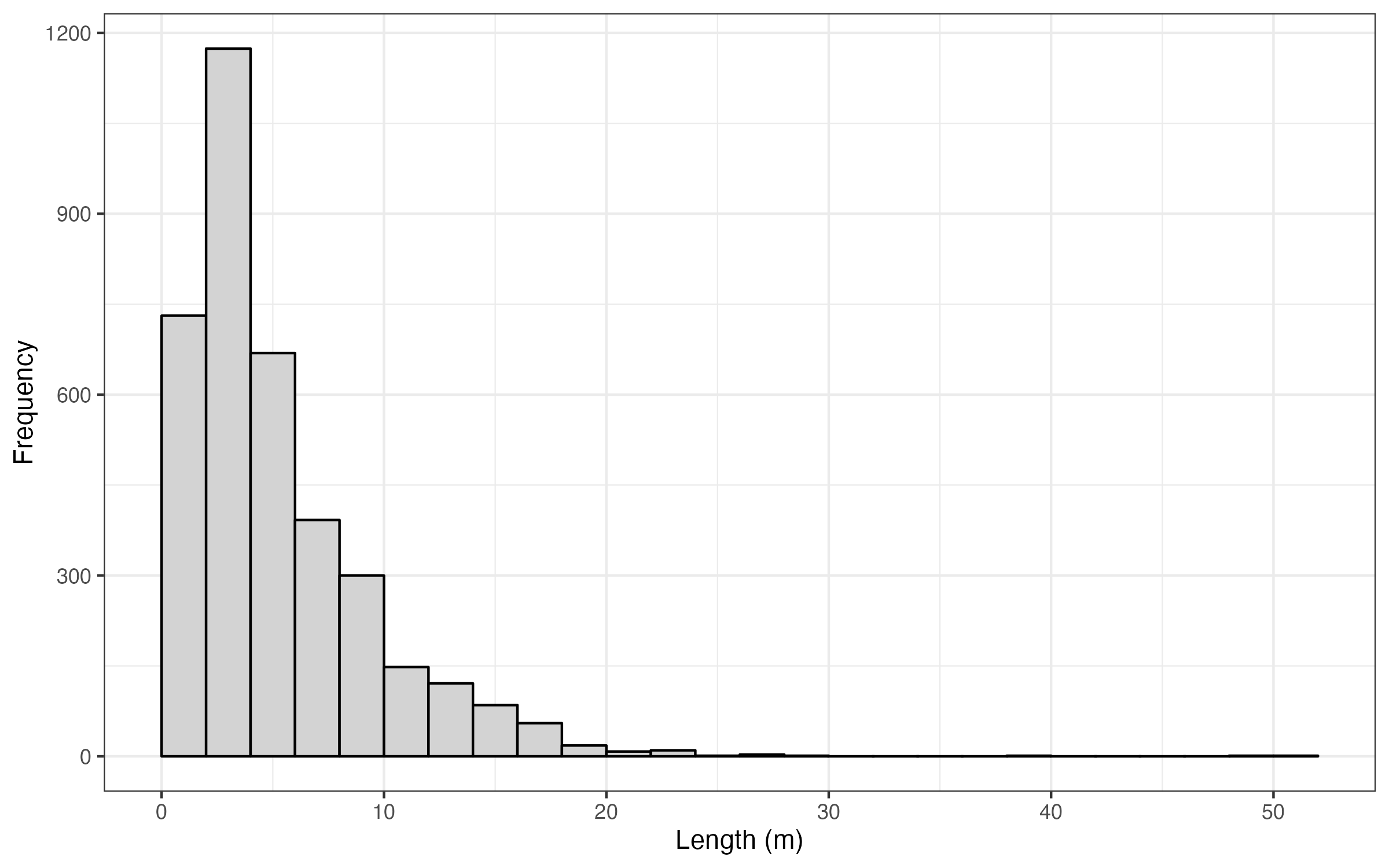
The mean error length was 5.2 m +/- 4.245 m SD, median = 3.9 m,
with a range of 0.067 m to 51 m.
Next, I binned the error vectors by angle, into 20 degree bins, and
calculated the sum of error lengths within each bin:
dat_length_bin <- dat_angle %>%
mutate(angle_bin = cut_width(angle_deg, 20, boundary = 0,
closed = "right")) %>%
group_by(angle_bin) %>%
summarise(
line_length_sum = sum(line_length)) %>%
mutate(angle_bin = as.numeric(gsub("\\[([0-9]+),.*", "\\1",
angle_bin)))
Then plotted a rose diagram of these summary data:
ggplot() +
geom_bar(data = dat_length_bin,
aes(x = angle_bin, y = line_length_sum),
stat = "identity", colour = "black", fill = "darkgrey",
width = 20,
position = position_nudge(x = 10)) +
coord_polar() +
scale_y_continuous(expand = c(0.1, 0)) +
scale_x_continuous(limits = c(0, 360), breaks = c(0, 90, 270,
360)) +
theme_bw() +
theme(
axis.text.y = element_blank(),
axis.ticks.y = element_blank())
labs(x = expression("Angle"~(degree)), y = "Total length (m)")
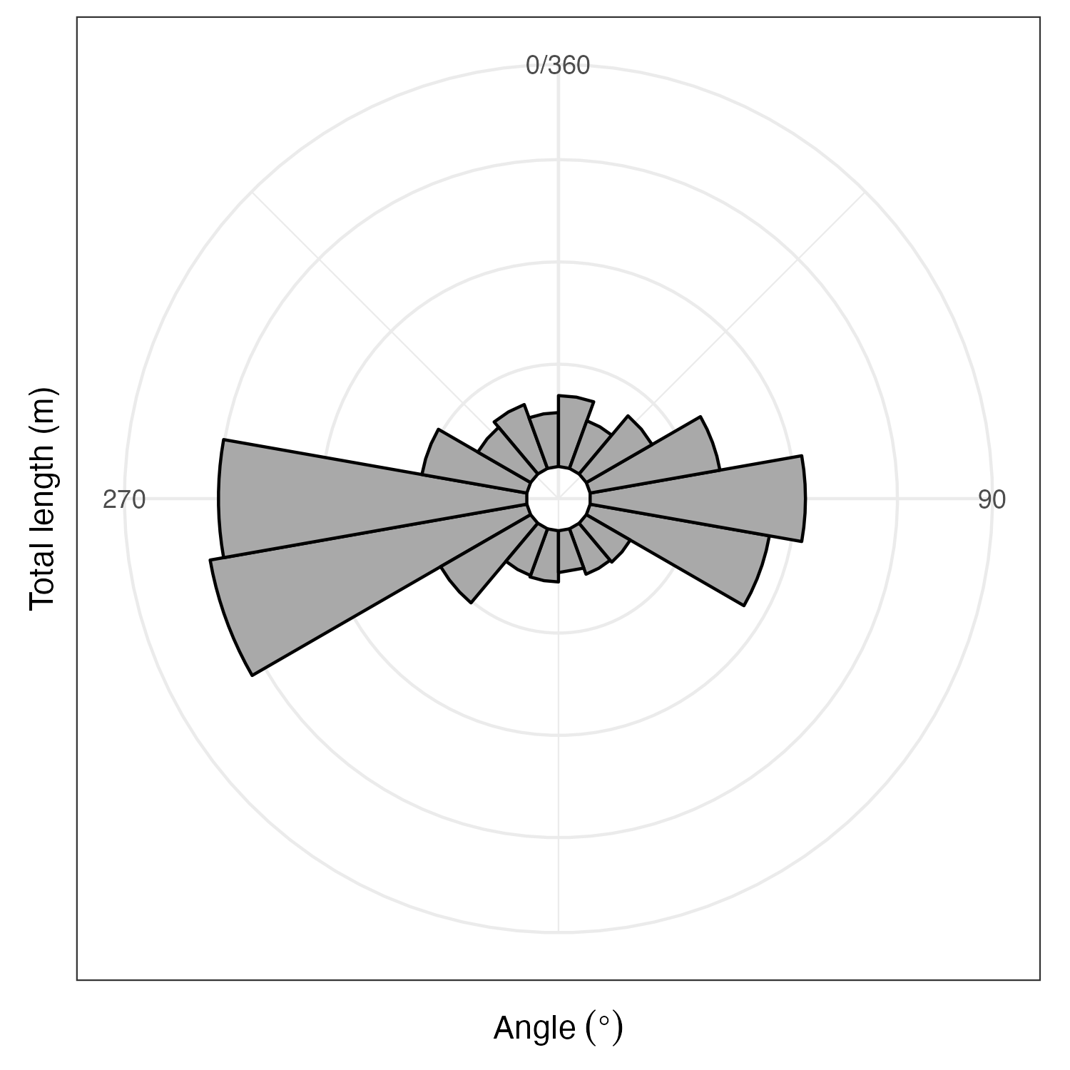
It looks like the biggest and most frequent errors are where the
grid coordinate is west of the GPS coordinate. This systematic
error probably has something to do with how we set up the tapes in
the plots, and represents error in the grid coordinates rather than
the GPS coordinates, as I'd expect the GPS coordinate error to be
random noise. It suggests that the person measuring the X axis
coordinate consistently over-estimated the position on the tape
measure, likely because they weren't holding the tapes perfectly
perpendicular.
The main problem with this comparison between GPS and tape measure
is that neither of these methods are guaranteed to provide the
truth. There is random error in the GPS points, handheld GPS units
are only accurate to about 2-3 m. However, there are also errors in
the tape measure method:
Firstly, the edges of the plot might not be totally square. The XY
coordinate system relies on the corners of the plot having a
perfect 90 degree angle, and each edge being a perfectly straight
line, but in the field this is difficult to achieve. Sometimes the
plots come out slightly rhombic, despite our best efforts.
It's also common for the tape measures to bow slightly in or out of
the plot. If the edge bows in, the distance from the plot edge to a
stem will be less in the middle of the plot than at the edges of
the plot. This is a particularly problem in a grassy plot on a
windy day, as the grass moves the tape measure. The only way to
stop this is to place the tape measure very close to the ground and
to anchor the tape measure at regular intervals.
The tape measures may stretch slightly leading to an under-estimate
of the measurement.
The tape measures may not be laid out perfectly parallel to the
plot edges. A tape measure laid out at an angle will increase the
measured length. Using smaller strips along the X axis in the
field, 10 m rather than 20 m, can reduce this error, as angle
errors result in larger location erors with increased distance.
Finally, there may be reporting errors in the field, and there may
be transcription errors when typing the data up onto the computer.
Commonly decimal points are put in the wrong place, or 65.6 m gets
called out as 45.6 m, when we move to a new row.
Where the goal is just to aid relocation of stems in future
censuses, I would definitely advocate for using a GPS unit. It
saves a lot of time, and the location accuracy is good enough.
Where it's necessary to quantify neighbourhood effects, I think
tape measures can probably give better accuracy and higher
precision, but only if the measuring is done by a trained team
working meticuluously, and the plot is set up properly to begin
with.
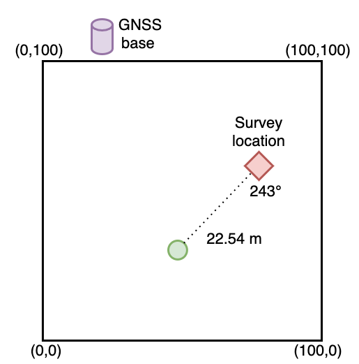
Another option for measuring tree location that I've been toying
with for a long time is using a laser total station or a laser
level in conjunction with differential GPS. Something like the
Leica NA520 which can measure angle and distance to a reflective
target. First you would pick a spot where many stems are visible
and set up a survey tripod. Then using a differential GPS system
you would record the precise location of the tripod. This could
take a few minutes, but only has to be done once for each batch of
measurements. Then the GPS antenna would be swapped out for a laser
level. The distance and angle of each stem in view with respect to
the level would be recorded. The survey tripod would be moved to
the next surveying location and the process would be repeated. Then
the location of each stem can be calculated using the real-space
location of the survey tripod, the angle and distance of the stem
with respect to the tripod. You could even record the same stem
multiple times from different positions to further improve the
accuracy of the location, but I think even for measuring
neighbourhood effects it's only really necessary to have an
accuracy of about 50-100 cm.
[Leica NA520]:
https://leica-geosystems.com/en-gb/products/levels/automatic-levels/
leica-na500-series