TITLE: Network graph of R package usage
DATE: 2021-06-25
AUTHOR: John L. Godlee
====================================================================
I wanted to know which R packages I use the most in my work, just
as a little toy exercise in data wrangling and network
visualisation.
I searched through all the R scripts on my laptop using ripgrep, to
find which packages I use:
[ripgrep]:
https://github.com/BurntSushi/ripgrep
rg "^library(.*)$" -g *.R -g '!Library/*' > packages.txt
The -g glob excludes any files in ~/Library, because these are
email attachments which sometimes aren't mine, and when they are
mine they're often duplicates of a script already stored on my
computer somewhere else.
Then in R, I can import the results and start analysing them:
# Packages
library(dplyr)
library(ggplot2)
library(GGally)
library(network)
# Import data
dat_raw <- readLines("packages.txt")
The first thing is to separate the filepaths from the package names:
# Extract file paths from lines
paths <- gsub(":.*", "", dat_raw)
# Check all paths are valid
stopifnot(all(grepl(".R$", paths)))
# Extract packages from lines
packages <- gsub(".*library\\s?\\(\"?([A-z0-9.]+)\"?\\).*",
"\\1", dat_raw)
# Check number of paths = number of packages
stopifnot(length(paths) == length(packages))
# Create dataframe
dat <- unique(data.frame(paths, packages))
The unique() removes some packages which were mistakenly called
multiple times in the same script.
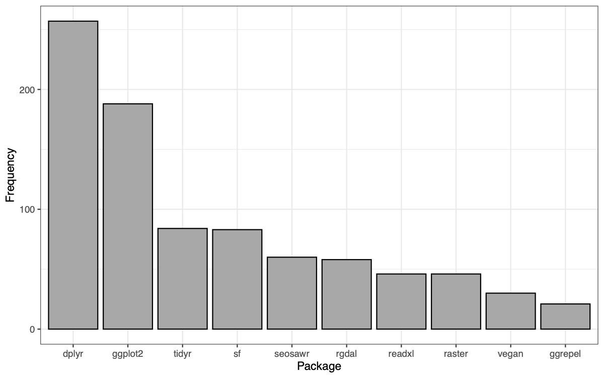
To find my most used packages, I created a bar graph:
pack_freq_summ <- dat %>%
group_by(packages) %>%
tally() %>%
mutate(packages = factor(packages, levels =
rev(packages[order(n)]))) %>%
arrange(desc(n)) %>%
slice_head(n = 10)
ggplot() +
geom_bar(data = pack_freq_summ,
aes(x = packages, y = n),
colour = "black", fill = "darkgrey", stat = "identity") +
theme_bw() +
labs(x = "Package", y = "Frequency")
Next, I wanted to create a network graph. I wanted to visualise
which packages were used the most, which packages were used in
conjunction with each other, and which packages are most commonly
used in conjunction.
First, split the dataframe by R script, and remove scripts which
only called one package.
# Split by file
dat_split <- split(dat, dat$paths)
# Remove files with only one package
dat_split_fil <- dat_split[unlist(lapply(dat_split, nrow)) > 1]
Then for each R script, use expand.grid() to create pairwise
combinations of packages and count their frequency, then use some
{dplyr} to clean up the results, so I'm left with a dataframe with
three columns, from, to, and weight, where from and to are pairs of
packages, and weight counts the number of times they are called in
the same script:
# Create matrix of packages by co-occurrence in files
edge_mat <- do.call(rbind, lapply(dat_split_fil, function(x) {
expand.grid(x$packages, x$packages)
})) %>%
filter(Var1 != Var2) %>%
group_by(Var1, Var2) %>%
tally() %>%
rename(from = Var1, to = Var2, weight = n) %>%
mutate(
from = as.character(from),
to = as.character(to)) %>%
group_by(grp = paste(pmax(from, to), pmin(from, to), sep =
"_")) %>%
slice(1) %>%
ungroup() %>%
select(-grp)
Then, I create a network object and add attributes so that the
nodes are weighted by frequency, and the edges are weighted by
co-occurrence frequency:
# Create network object
net <- as.network(edge_mat, directed = FALSE)
# Add vertex attribute, number of times package is used
vertex_weight <- dat %>%
group_by(packages) %>%
tally() %>%
as.data.frame()
net %v% "vweight" <- vertex_weight[
match(net %v% "vertex.names", vertex_weight$packages),"n"]
# Add edge attribute, colors by number of times packages used
in conjunction
colfunc <- colorRampPalette(c("lightgray", "blue"))
net %e% "edgecol" <- as.character(cut(
log(net %e% "weight"), breaks = 5, labels = colfunc(5)))
And finally, create a circular network graph, where nodes are sized
according to frequency and edges are coloured according to
co-occurrence frequency:
# Create plot
ggnet2(net, mode = "circle",
color = "#ffc780", size = "vweight",
label = TRUE, label.size = 2,
edge.col = "edgecol")
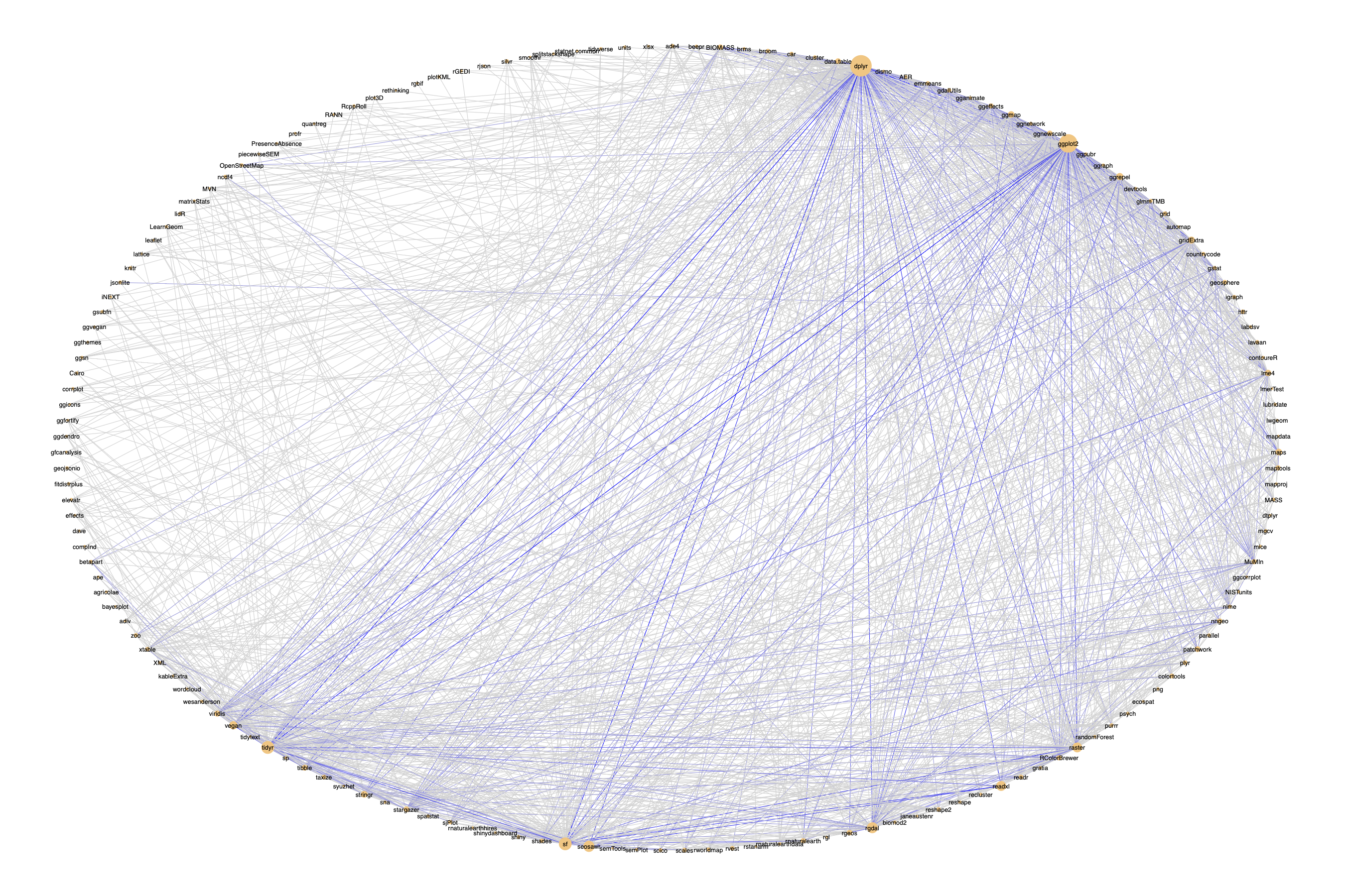
I'm not totally happy with the edge colouring, but it's difficult
because many packages only occur together once, while a few, e.g.
{dplyr} occur in almost every script, so there's a very wide range
of values.