TITLE: Calculating the winkelmass in R
DATE: 2021-05-10
AUTHOR: John L. Godlee
====================================================================
Winkelmass means "angle measure" in German. In forestry the term
has been adopted to refer to a specific metric used to describe the
regularity of tree spatial distribution. Literature on the
winkelmass traces mostly to Klaus von Gadow, a researcher split
between the University of Göttingen and Beijing Forestry
University. The winkelmass is quite simple at it's core. For each
tree, a given number of nearest neighbours are identified, usually
four. Then, going clockwise around the focal tree, the angle
between each neighbour and the next neighbour is calculated. For
each angle, if the angle is less than the 'critical angle' i.e. 360
degrees divided by the number of neighbours considered, a value of
1 is recorded, otherwise, a value of 0 is recorded. Finally, the
sum of these values divided by the number of neighbours gives the
winkelmass. In LaTeX math:
W_{i} = \frac{1}{k} \sum_{j=1}^{k} v_{j}
where W is the winkelmass, k is the number of neighbours
considered, and v_{j} is either 0 or 1 depending on the angle
between two neighbours.
To calculate the plot-level winkelmass, simply take the mean of all
W_{i} values in the plot.
I wrote a function in R to calculate the Winkelmass for all trees
in a plot:
#' Winkelmass (spatial regularity of trees)
#'
#' @param x vector of individual x axis coordinates
#' @param y vector of individual y axis coordinates
#' @param k number of neighbours to consider
#'
#' @references von Gadow, K., Hui, G. Y. (2001). Characterising
forest spatial
#' structure and diversity. Sustainable Forestry in Temperate
Regions. Proc. of
#' an international workshop organized at the University of
Lund, Sweden.
#' Pages 20- 30.
#'
winkelmass <- function(x, y, k = 4) {
dat_sf <- sf::st_as_sf(data.frame(x,y), coords = c("x", "y"))
dists <- suppressMessages(nngeo::st_nn(dat_sf, dat_sf, k =
k+1,
progress = FALSE))
a0 <- 360 / k
wi <- unlist(lapply(dists, function(i) {
focal_sfg <- sf::st_geometry(dat_sf[i[1],])[[1]]
nb_sfg <- sf::st_geometry(dat_sf[i[-1],])
nb_angles <- sort(unlist(lapply(nb_sfg, function(j) {
angleCalc(focal_sfg, j)
})))
aj <- nb_angles - c(NA, head(nb_angles, -1))
aj[1] <- nb_angles[k] - nb_angles[1]
aj <- ifelse(aj > 180, 360 - aj, aj)
aj <- round(aj, 1)
sum(aj < a0)
}))
out <- 1 / k * wi
return(out)
}
The function uses {nngeo} to find nearest neighbours of each tree
by their x and y grid coordinates. Then it makes {sf} geometry
objects and calculates the angles between them, and finally does a
bit of arithmetic to find if the angles are less than the critical
angle. An important aspect to the calculation is that if the angle
between two neighbours is greater than 180 degrees, the opposite
angle is taken. So if an angle is 275 degrees, the recorded angle
is 360 - 275 = 85 degrees. In this example by taking the opposite
angle the value of v_{j} changes from 0 (275 gt 90) to 1 (85 lt 90).
The angleCalc() function is:
#' Calculate angle between two sf point objects
#'
#' @param x point feature of class 'sf'
#' @param y point feature of class 'sf'
#'
#' @return azimuthal from x to y, in degrees
#'
#' @examples
#' p1 <- st_point(c(0,1))
#' p2 <- st_point(c(1,2))
#' angleCalc(p1, p2)
#'
#' @export
#'
angleCalc <- function(x, y) {
dst_diff <- as.numeric(x - y)
return((atan2(dst_diff[1], dst_diff[2]) + pi) / 0.01745329)
}
I also wrote some tests for the function to make sure it worked
properly. First, packages, all for visualising results, not needed
for calculations:
library(ggplot2)
library(patchwork)
library(knitr)
Define a function to create maps to visualise the distribution of
neighbours around a focal tree:
linemake <- function(dat) {
out <- data.frame(
xmin = rep(dat$x[1], times = nrow(dat) - 1),
ymin = rep(dat$y[1], times = nrow(dat) - 1),
xmax = dat$x[-1], ymax = dat$y[-1])
return(out)
}
plotmake <- function(dat) {
lout <- linemake(dat)
dat$label <- c("F", "1", "2", "3", "4")
ggplot() +
geom_segment(data = lout,
aes(x = xmin, y = ymin, xend = xmax, yend = ymax)) +
geom_label(data = dat, aes(x = x, y = y, label = label)) +
coord_equal() +
theme_classic() +
labs(x = "X", y = "Y")
}
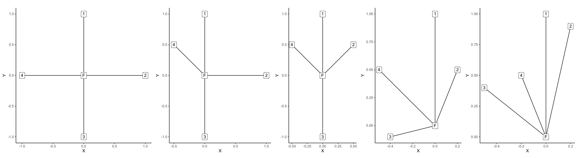
Create a number of test cases with different spatial distributions
of neighbours. Each test case should produce a different value of
Wi for the focal tree.
test_list <- list(
test1 = data.frame(x = c(0,0,1,0,-1), y = c(0,1,0,-1,0)),
test2 = data.frame(x = c(0,0,1,0,-0.5), y =
c(0,1,0,-1,0.5)),
test3 = data.frame(x = c(0,0,0.5,0,-0.5), y =
c(0,1,0.5,-1,0.5)),
test4 = data.frame(x = c(0,0,0.2,-0.4,-0.5), y =
c(0,1,0.5,-0.1,0.5)),
test5 = data.frame(x = c(0,0,0.2,-0.5,-0.2), y =
c(0,1,0.9,0.4,0.5))
)
Create the maps to visualise layout of the test cases:
plot_list <- lapply(test_list, plotmake)
wrap_plots(plot_list) +
plot_layout(nrow = 1)
Finally run the winkelmass() function and extract the first value
which refers to the focal tree:
kable(
unlist(lapply(test_list, function(x) {
winkelmass(x$x, x$y)[1]
})))
Ex Wi
------- ------
test1 0.00
test2 0.25
test3 0.50
test4 0.75
test5 1.00
As you can see, for a given value of k, there are k+1 possible
values of Wi depending on the distribution of neighbours.