TITLE: Modelling stem diameter class distribution with Weibull
distributions
DATE: 2021-03-30
AUTHOR: John L. Godlee
====================================================================
The two-parameter Weibull probability distribution is commonly used
to model the distribution of stem diameters in forests. The scale
and shape parameters can be used to compare different forest stands
to see how their distributions vary. I created a function in R
which calculates these parameters per plot, basically a wrapper
around MASS::fitdistr(). It's worth noting that FPC refers to
adjustments by sampling effort that may occur in plots with a
nested sampling design:
#' Fit a two-parameter Weibull distribution of diameter size
classes
#'
#' @param x dataframe of stem measurements
#' @param plot_id column name string of plot IDs
#' @param diam column name string of stem diameters
#' @param fpc column name string of stem FPC values
#' @param return_fit logical, optionally return a list of model
objects instead
#' of a dataframe of parameters
#'
#' @return dataframe with the shape and scale parameters, and
the standard
#' errors of each parameter for each plot-level Weibull
distribution
#'
#' @details The two-parameter Weibull distribution is a
probability density
#' function of the form: \eqn{f(D) = c/d(D/d)^{c-1}
exp(–(D/d)^{c})},
#' where $c$ is the shape parameter, $d$ is the scale
parameter, and $D$
#' is the stem diameter. To deal with variation in sampling
effort, this
#' function duplicates rows based on their FPC, rounding
the number of rows
#' up or down. E.g. a stem with FPC=0.08 would be
duplicated 13 times,
#' because $1/0.08=12.5$. The Weibull distribution is
fitted here using
#' Maximum Likelihood. $c$ is closely related to the mean
stem diameter
#' in most cases. $d<1$ indicates a concave exponential
which becomes more
#' extreme as $d -> 0$, while $d>1$ indicates a hump-shaped
#' relationship which becomes increasingly left-skewed as
#' $d -> inf$.
#'
#' Note that the Weibull distribution is not capable of
representing
#' bimodal or more complex diameter distributions, which
can occur in
#' disturbed woodlands.
#'
#' Any NA diameters will be excluded from the calculation
#'
#' @examples
#'
#' @importFrom MASS fitdistr
#'
#' @export
#'
diamWeibullGen <- function(x, plot_id = "plot_id", diam =
"diam", fpc = "fpc",
return_fit = FALSE) {
x_split <- split(x, x[[plot_id]])
out <- lapply(x_split, function(y) {
y_dup <- y[rep(row.names(y), round(1 / y[[fpc]])),]
y_fil <- y_dup[!is.na(y_dup[[diam]]),]
fit <- tryCatch({
suppressWarnings(MASS::fitdistr(y_fil[[diam]], "weibull"))
},
error = function(cond) {
return(NA)
})
if (return_fit) {
ret <- fit
} else {
if (!is.list(fit)) {
ret <- data.frame(
weibull_shape = NA,
weibull_scale = NA,
weibull_shape_se = NA,
weibull_scale_se = NA,
plot_id = unique(y[[plot_id]])
)
} else {
ret <- data.frame(
weibull_shape = fit[[1]][1],
weibull_scale = fit[[1]][2],
weibull_shape_se = fit[[2]][1],
weibull_scale_se = fit[[2]][2],
plot_id = unique(y[[plot_id]])
)
}
}
ret
})
if (!return_fit) {
out <- do.call(rbind, out)
names(out)[names(out) == "plot_id"] <- plot_id
}
return(out)
}
I created another function which fits a Weibull distribution and
extrapolates it to estimate the number of stems within arbitrary
size classes:
#' Estimate lower size-class abundances in plots with higher
minimum diameter thresholds
#'
#' @param x dataframe of stem measurements
#' @param plot_data dataframe of plot data
#' @param binwidth
#' @param min_diam_thresh column name string of minimum
diameter threshold in \code{plot_data}
#' @param diam column name string of stem diameter in \code{x}
#' @param min_limit lower diameter limit down to which to
estimate stem abundance
#' @param size_classes vector of size classes
#'
#' @return dataframe of stem abundances per size class
#'
#' @examples
#'
#'
#' @export
#'
diamWeibullEst <- function(x, plot_data, bins,
stem_plot_id = "plot_id", plot_plot_id = stem_plot_id,
min_diam_thresh = "min_diam_thresh", diam = "diam", fpc =
"fpc") {
# Get plot IDs in stems and plots
plots_all <- unique(c(x[[stem_plot_id]],
plot_data[[plot_plot_id]]))
# Which plot IDs are shared?
good_plots <- plots_all[plots_all %in% x[[stem_plot_id]] &
plots_all %in% plot_data[[plot_plot_id]]]
# Plots not in stems
plots_not_in_stems <- plots_all[!plots_all %in%
x[[stem_plot_id]]]
# Plots not in plots
plots_not_in_plots <- plots_all[!plots_all %in%
plot_data[[plot_plot_id]]]
# Plots with no min diam thresh
plot_no_thresh <-
plot_data[is.na(plot_data[[min_diam_thresh]]), plot_plot_id]
# Warning for plots with no min diam thresh
seosawr:::warnFormat(plot_no_thresh,
"Some plots have NA diameter thresholds:", "warning", 15)
# Warning for any plots which have been dropped
seosawr:::warnFormat(plots_not_in_plots,
"Some plots not present in plot data, will be NA:",
"warning", 15)
seosawr:::warnFormat(plots_not_in_stems,
"Some plots have no stems, will be 0:", "warning", 15)
# For each plot
out <- do.call(rbind, lapply(plots_all, function(y) {
# Get stems and plots
x_fil <- x[x[[stem_plot_id]] == y & !is.na(x[[diam]]),]
plots_fil <- plot_data[plot_data[[plot_plot_id]] == y,]
# Find min diam thresh
if (nrow(plots_fil) > 0) {
min_diam <- min(plots_fil[[min_diam_thresh]], na.rm =
TRUE)
# Filter to plot diameter threshold
x_fil <- x_fil[x_fil[[diam]] >= min_diam &
!is.na(x_fil[[diam]]),]
# Calculate weibull
if (nrow(x_fil) > 0) {
weib <- diamWeibullGen(x_fil, diam = diam, plot_id =
stem_plot_id,
fpc = "fpc", return_fit = FALSE)
# Get replicated rows by FPC
x_dup <- x_fil[rep(row.names(x_fil), round(1 /
x_fil[[fpc]])),]
# Extract Weibull parameters
weib_shape <- weib$weibull_shape
weib_scale <- weib$weibull_scale
# Find number of stems used to generate the
distribution
nstems_obs <- length(x_dup[[diam]])
# Find predicted proportion of stems this represents
prop_obs <- unname(exp(-(min_diam /
weib_scale)^weib_shape))
# Estimate total number of stems
nstems_total <- nstems_obs / prop_obs
# For each bin, calculate estimated proportion of
stems
n_est <- unlist(lapply(bins, function(z) {
# Estimate proportion of stems in category of
interest
prop_cat <- unname(exp(-(z[[1]] /
weib_scale)^weib_shape) -
exp(-(z[[2]] / weib_scale)^weib_shape))
prop_cat * nstems_total
}))
} else {
n_est <- 0
}
} else {
n_est <- NA_real_
}
# Create pretty bin chars
diam_class <- unlist(lapply(bins, function(z) {
paste(z[[1]], z[[2]], sep = "-")
}))
# Create dataframe of output
ret <- data.frame(y, diam_class, n_est)
names(ret)[1] <- plot_plot_id
# Return
ret
}))
# Return
return(out)
}
The function models stem numbers reasonably consistently among
plots, but tends to under-estimate the lower diameter size classes:
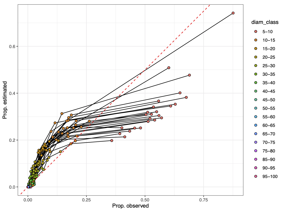
In the plot each set of points connected by a line is a plot, and
each point is a diameter size class, with the proportion of stems
observed within that size class on the x axis, and the proportion
of stems estimated by diamWeibullEst() on the y axis. As you can
see, large diameter size classes are slightly over-estimated in
their proportional abundance, and the smallest size class (5-10 cm)
is consistently under-estimated. This is probably because the
Weibull distribution will dip down towards zero unless the shape
parameter (k) is less than 1.