TITLE: Estimating canopy rugosity from terrestrial LiDAR
DATE: 2021-01-01
AUTHOR: John L. Godlee
====================================================================
As part of my PhD research I have been using terrestrial LiDAR to
understand woodland tree canopy traits in southern African
savannas. One of the measurements I wanted to make was an estimate
of the roughness of the top of the canopy. I've also heard this
referred to as the canopy rugosity. In a previous post I've already
described how I processed the raw point cloud data to produce a
csv with XYZ point coordinates, so I'll skip straight to how I
used R to estimate canopy rugosity.
After reading in the file with data.table::fread() the first thing
was to assign each point to a 10x10cm 2D bin in the XY plane, then
I took the 95th percentile, 99th percentile, and maximum point
height within each bin:
dat <- fread(x)
# Assign each point to a 2D bin,
# 10x10 cm bins
dat_xy_bin <- dat %>%
mutate(
bin_x = cut(.$X, include.lowest = TRUE, labels = FALSE,
breaks = seq(floor(min(.$X)), ceiling(max(.$X)), by =
xy_width)),
bin_y = cut(.$Y, include.lowest = TRUE, labels = FALSE,
breaks = seq(floor(min(.$Y)), ceiling(max(.$Y)), by =
xy_width)))
# Quantiles of height in each bin
dat_xy_bin_summ <- dat_xy_bin %>%
group_by(bin_x, bin_y) %>%
summarise(
q95 = quantile(Z, 0.95),
q99 = quantile(Z, 0.99),
max = max(Z, na.rm = TRUE)
)
Then I extracted a number of simple descriptive statistics from the
distributions of values (q95, q99, max) across each XY bin:
- Mean
- Median
- Standard deviation
- Range
- Coefficient of variation (StDev / mean * 100)
- Modal 10cm height bin
# Calculate mean, median, stdev of distribution (canopy top
rugosity)
summ <- dat_xy_bin_summ %>%
ungroup() %>%
summarise(across(c(q95, q99, max),
list(
max = ~max(.x, na.rm = TRUE),
min = ~min(.x, na.rm = TRUE),
mean = ~mean(.x, na.rm = TRUE),
median = ~median(.x, na.rm = TRUE),
sd = ~sd(.x, na.rm = TRUE),
range = ~max(.x, na.rm = TRUE) - min(.x, na.rm = TRUE),
cov = ~sd(.x, na.rm = TRUE) / mean(.x, na.rm = TRUE) *
100,
median_max_ratio = ~median(.x, na.rm = TRUE) / max(.x,
na.rm = TRUE),
mode_bin = ~as.numeric(
gsub("]", "",
gsub(".*,", "",
names(sort(table(cut(.x,
seq(floor(min(.x)),
ceiling(max(.x)), by = xy_width))),
decreasing = TRUE)[1]))))
))) %>%
gather() %>%
mutate(plot_id = plot_id) %>%
dplyr::select(plot_id, key, value) %>%
bind_rows(.,
data.frame(plot_id = plot_id, key = "entropy",
value = enl(dat$Z, z_width)))
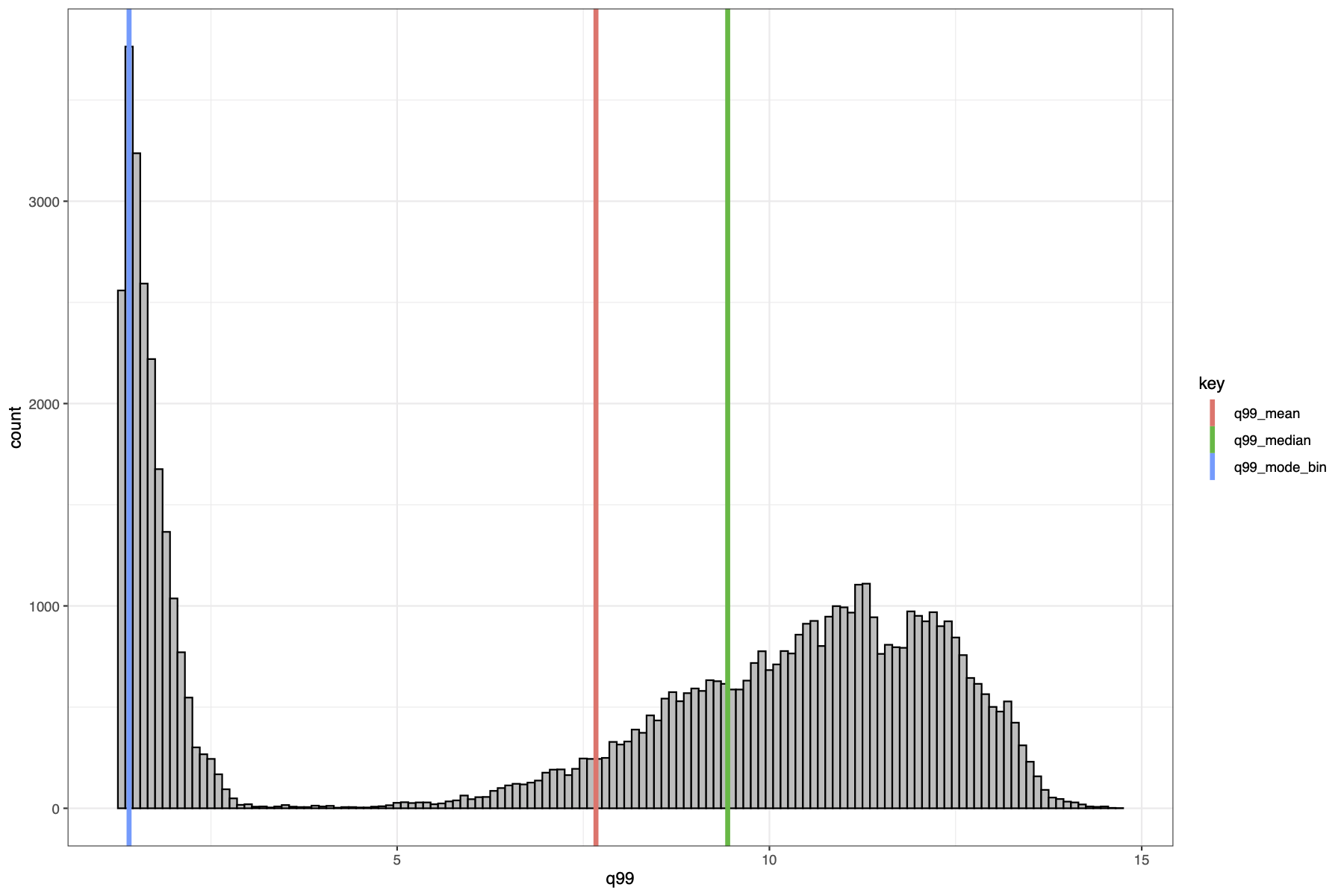
Finally I made a histogram of the canopy top distribution, and a
surface plot of the canopy height surface:
# Histogram of distribution
pdf(file = file.path("../img/canopy_height_hist",
paste0(plot_id, "_canopy_height_hist.pdf")), width = 12,
height = 8)
print(
ggplot() +
geom_histogram(data = dat_xy_bin_summ, aes(x = q99), binwidth =
xy_width,
fill = "grey", colour = "black") +
geom_vline(data = summ[summ$key %in% c("q99_mode_bin",
"q99_mean", "q99_median"),],
aes(xintercept = value, colour = key),
size = 1.5) +
theme_bw()
)
dev.off()
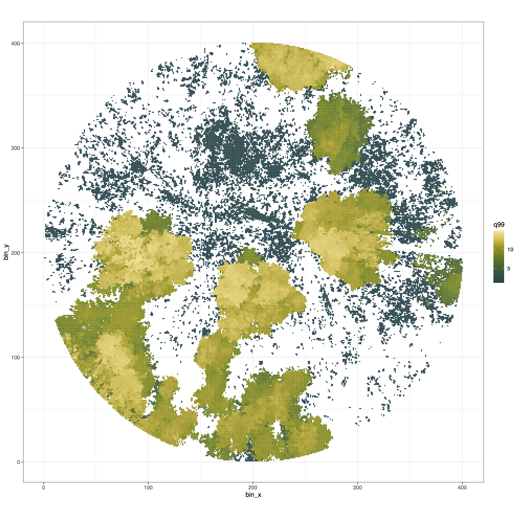
# Surface plot of canopy height surface
pdf(file = file.path("../img/canopy_height_surface",
paste0(plot_id, "_canopy_height_surface.pdf")), width = 12,
height = 12)
print(
ggplot() +
geom_tile(data = dat_xy_bin_summ,
aes(x = bin_x, y = bin_y, fill = q99)) +
scale_fill_scico(palette = "bamako") +
theme_bw() +
coord_equal()
)
dev.off()