TITLE: Extracting a vertical height profile from terrestrial LiDAR
DATE: 2020-12-30
AUTHOR: John L. Godlee
====================================================================
Previously, measuring canopy cover with hemispherical photography
only provided a 2D representation of the canopy, but with LiDAR
it's possible to measure variation in canopy cover over the height
of the canopy to create a canopy height profile. Here I want to
describe how I used R to process the XYZ point cloud data to create
a canopy height profile. I have already described in a previous
post how I voxelise, clean and crop the point cloud, using PDAL.
[PDAL]:
https://pdal.io/
# Packages
library(ggplot2)
library(dplyr)
library(data.table)
library(scico)
library(zoo)
I used data.table::fread() to read the XYZ point cloud .csv files
into R, as they are very large, about 500 MB, and fread() seems to
do a better job at reading large files into memory.
For each file, I rounded the elevation (Z) coordinates to the
nearest cm, then for each cm height bin I calculated the volume of
space occupied by voxels.
I created a height foliage density profile with ggplot().
I calculated the effective number of layers according to Ehbrecht
et al. 2016 (Forest Ecology and Management), which basically splits
the height profile into 1 m bins and calculates the Shannon
diversity index of the foliage volume occupied in each layer. Here
is the function for it:
#' Effective number of layers in a point cloud distribution
#'
#' @param x vector of Z (elevation) coordinates
#' @param binwidth width of vertical bins in units of x
#'
#' @return atomic vector of length one describing the effective
number of layers
#' in the canopy
#'
#' @details Uses the Shannon diversity index (Entropy) to
estimate the
#' "Effective Number of Layers" in the vertical profile of
a point cloud
#' distribution.
#'
#' @references
#' Martin Ehbrecht, Peter Schall, Julia Juchheim, Christian
Ammer, &
#' Dominik Seidel (2016). Effective number of layers: A new
measure for
#' quantifying three-dimensional stand structure based on
sampling with
#' terrestrial LiDARForest Ecology and Management, 380,
212–223.
#'
#' @examples
#' x <- rnorm(10000)
#' enl(x)
#'
# Calculate effective number of layers in canopy
## Assign to Z slices
## Count number of points within each slice
## Calculate shannon diversity index (entropy) on vertical
layer occupancy
enl <- function(x, binwidth) {
binz <- cut(x, include.lowest = TRUE, labels = FALSE,
breaks = seq(floor(min(x)), ceiling(max(x)), by =
binwidth))
n <- unlist(lapply(split(x, binz), length))
entropy <- exp(-sum(n / sum(n) * log(n / sum(n))))
return(entropy)
}
I calculated the area under the curve of the foliage density
profile using density() then zoo::rollmean(), a method I stole of
Stack Overflow.
I also calculated the height above the ground of the peak of
foliage density.
Here is the script in its entirety:
# Import data
file_list <- list.files(path = "../dat/tls/height_profile",
pattern = "*.csv",
full.names = TRUE)
# Check for output directories
hist_dir <- "../img/foliage_profile"
if (!dir.exists(hist_dir)) {
dir.create(hist_dir, recursive = TRUE)
}
out_dir <- "../dat/subplot_profile"
if (!dir.exists(out_dir)) {
dir.create(out_dir, recursive = TRUE)
}
# Define parameters
voxel_dim <- 0.01
z_width <- 1
cylinder_radius <- 10
# Calculate maximum 1 voxel layer volume
layer_vol <- pi * cylinder_radius^2 * voxel_dim
# For each subplot:
profile_stat_list <- lapply(file_list, function(x) {
# Get names of subplots from filenames
subplot_id <- gsub("_.*.csv", "", basename(x))
plot_id <- gsub("(^[A-Z][0-9]+).*", "\\1", subplot_id)
subplot <- gsub("^[A-Z][0-9]+(.*)", "\\1", subplot_id)
# Read file
dat <- fread(x)
# Round Z coords to cm
dat$z_round <- round(dat$Z, digits = 2)
# Calculate volume and gap fraction
bin_tally <- dat %>%
group_by(z_round) %>%
filter(z_round > 0) %>%
tally() %>%
as.data.frame() %>%
mutate(vol = n * voxel_dim,
gap_frac = vol / layer_vol)
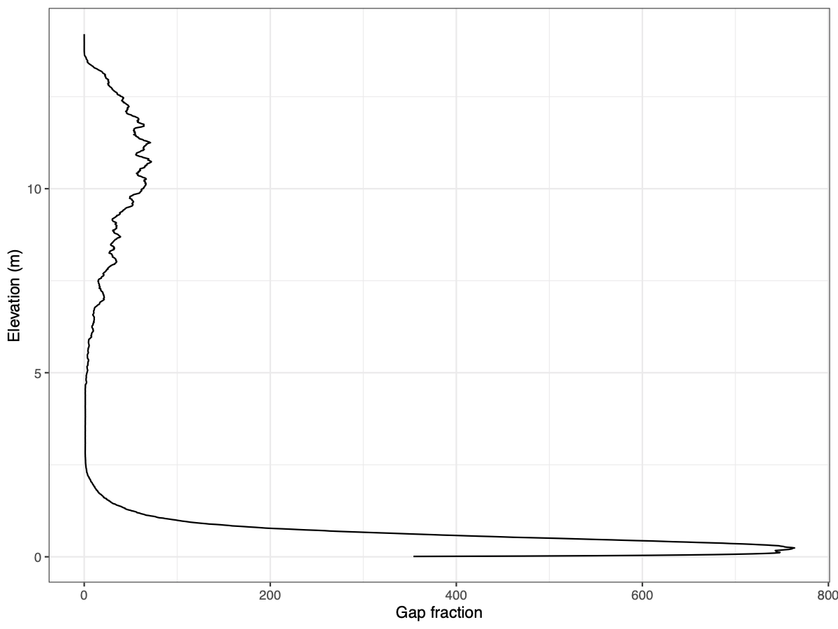
# Plot gap fraction density plot
pdf(file = paste0(hist_dir, "/", subplot_id,
"_foliage_profile.pdf"),
width = 8, height = 6)
print(
ggplot(bin_tally, aes(x = z_round, y = gap_frac)) +
geom_line() +
theme_bw() +
labs(x = "Elevation (m)", y = "Gap fraction") +
coord_flip()
)
dev.off()
# Calculate effective number of layers
layer_div <- enl(dat$Z, z_width)
# Calculate area under curve
den <- density(dat$z_round)
den_df <- data.frame(x = den$x, y = den$y)
auc_canopy <- sum(diff(den_df$x) * rollmean(den_df$y, 2))
# Calculate height of max peak
dens_peak_height <- den_df[den_df$y == max(den_df$y), "x"]
# Create dataframe from stats
out <- data.frame(plot_id, subplot, layer_div, auc_canopy,
dens_peak_height)
# Write to file
write.csv(out,
file.path(out_dir,
paste0(paste(plot_id, subplot, sep = "_"), "_summ.csv")),
row.names = FALSE)
return(out)
})