TITLE: Measuring canopy gap fraction from point clouds
DATE: 2020-12-20
AUTHOR: John L. Godlee
====================================================================
For my PhD research I wanted to estimate woodland canopy traits to
see how they vary with species composition at my field site in
southwest Angola. In the past I've used hemispherical photography
to estimate canopy gap fraction, measured as the percentage of the
sky hemisphere covered by plant material. This time however, I had
a terrestrial laser scanner and I wanted to compare how the
hemispherical photography method compared to the terrestrial laser
scanner.
With the laser scanner I used (Leica HDS6100) it's fairly easy to
estimate canopy gap fraction from a single scan as it has a
hemispherical line of sight. It's simply a case of counting the
number of laser pulses which didn't bounce off a plant and return
to the scanner, then expressing that as a propotion of the total
number of pulses emitted.
In my case however, I wanted to make a few different measurements
of small plots, and some of those measurements require a point
cloud with no shadows, that is, a 3D model of the plot where all
surfaces within the plot have been scanned at least once. With only
one scan, a tree trunk near to the scanner can block the view to
everything behind it, which can bias the results. To create a
shadow-less point cloud one must move the laser scanner around
within the plot and make multiple scans which are then stitched
back together. This means that the centre of the plot, where the
hemispherical photograph was taken, doesn't match up with the
centre of the point cloud.
I decided to simulate a hemispherical photograph using the point
cloud data and compare that to the hemispherical photo.
In a previous post I described how I processed the .ptx raw point
cloud data to make it easier for further analysis so I won't focus
on it here.
First, I had to take the voxelised point cloud and centre it on the
centre of the subplot, using coordinates which I recorded with a
differential GPS system. I used PDAL for this, along with some AWK
and shell scripting to automate the process for many plots with
different coordinates.
[PDAL]:
https://pdal.io/
I used this script to extract latitude and longitude from a .csv
with plot centres defined by a plot ID.
awk -v SUBPLOT="$1" 'BEGIN { FPAT = "([^,]+)|(\"[^\"]+\")" }
$5 ~ SUBPLOT && $14 == "TRUE" {printf "%f\n%f\n", $6, $7}'
./dat/target_coords.csv
Then I used a shell script connected to a PDAL pipeline to centre
the point cloud:
#!/usr/bin/env sh
if [ $# -lt 4 ]; then
printf "Must supply at least four arguments\n [1]
input.laz\n [2] longitude\n [3] latitude\n [4] output.laz\n"
exit 1
fi
noext="${i%_*.laz}"
matrix="1 0 0 -$2 0 1 0 -$3 0 0 1 0 0 0 0 1"
pdal pipeline pipelines/centre.json --readers.las.filename=$1 \
--filters.transformation.matrix="${matrix}" \
--writers.las.filename=$4
and here is the JSON pipeline:
[
{
"type" : "readers.las",
"filename" : "input.laz"
},
{
"type" : "filters.transformation",
"matrix" : "0 -1 0 1 1 0 0 2 0 0 1 3 0 0 0
1"
},
{
"type" : "writers.las",
"compression" : "true",
"minor_version" : "2",
"dataformat_id" : "0",
"forward" : "all",
"filename" : "output.laz"
}
]
Then I cropped the point cloud to a cylinder of 20 m diameter,
again with a PDAL pipeline:
[
{
"type" : "readers.las",
"filename" : "input.las"
},
{
"type" : "filters.crop",
"point" : "POINT(0 0)",
"distance" : 20
},
{
"type" : "writers.las",
"compression" : "true",
"minor_version" : "2",
"dataformat_id" : "0",
"forward" : "all",
"filename" : "output.laz"
}
]
I classified ground points and reset the height of the point cloud
based on the ground classification, then subsetted to only points
above 1.3 m, which is the height the hemispherical photo was taken:
[
{
"type" : "readers.las",
"filename" : "input.laz"
},
{
"type" : "filters.pmf"
},
{
"type" : "filters.hag_nn",
"allow_extrapolation" : "true"
},
{
"type":"filters.ferry",
"dimensions":"HeightAboveGround=>Z"
},
{
"type" : "filters.range",
"limits" : "Z[1.3:]"
},
{
"type" : "writers.las",
"compression" : "true",
"minor_version" : "2",
"dataformat_id" : "0",
"forward" : "all",
"filename" : "output.laz"
}
]
I then converted the point cloud to a .csv of XYZ coordinates, one
point per row:
[
{
"type" : "readers.las",
"filename" : "input.laz"
},
{
"type" : "writers.text",
"format" : "csv",
"precision" : 3,
"order" : "X,Y,Z",
"keep_unspecified" : "false",
"filename" : "output.csv"
}
]
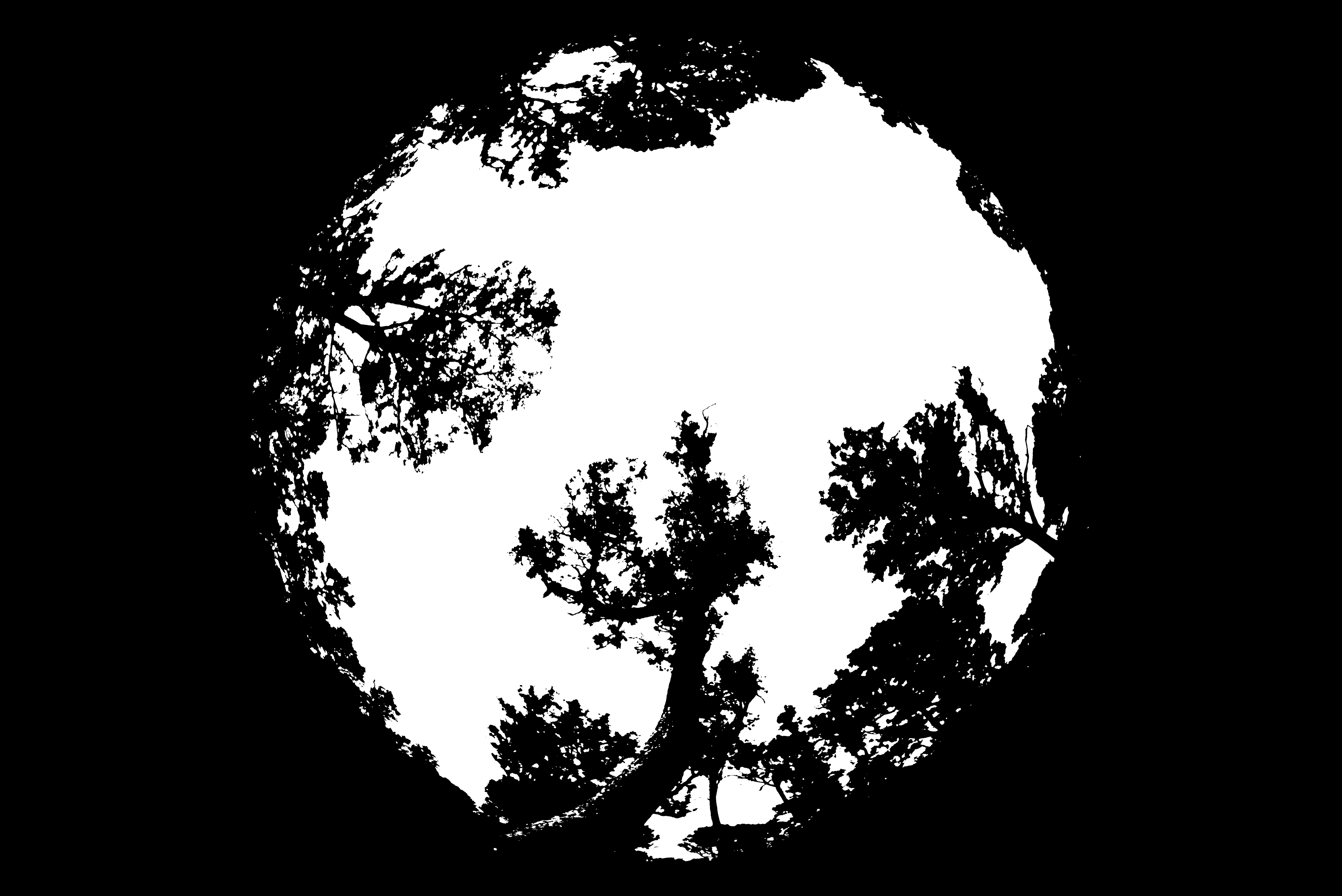
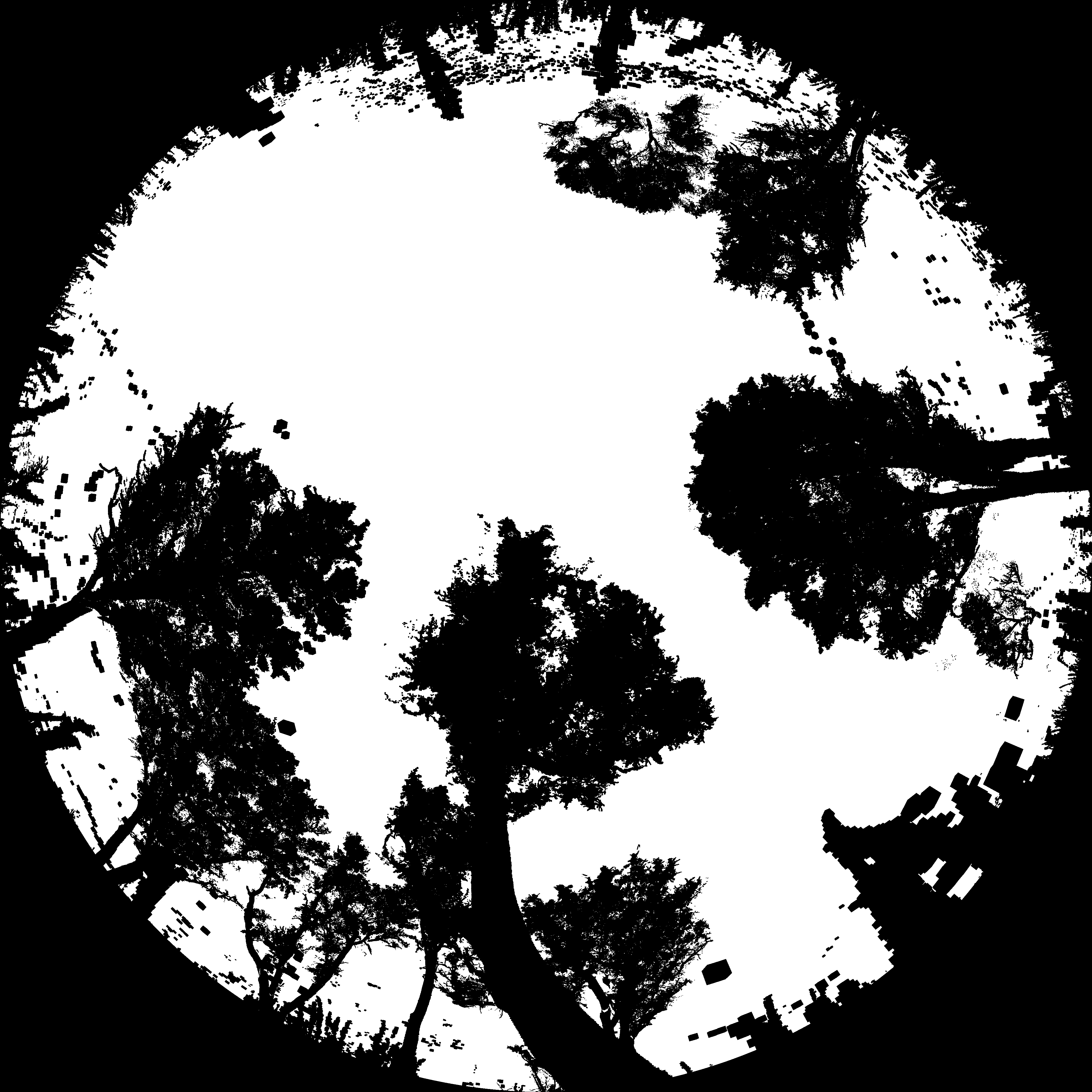
The interesting bit is next. I used a program called POV-ray to
draw voxels in a 3D space at the position of each point in the
point cloud and with the same size as the voxels defined during
voxelisation. Then I positioned a virtual camera pointing upwards
at the subplot centre, the same setup and lens curvature as the
hemispherical photograph, with a white sky and black voxels, to
create a virtual hemispherical photograph. Here is a side by side
comparison of a real hemispherical photo (top) and a virtual photo
(bottom) from a single plot. Note that the real photo is a mirror
image, as you would expect from a photo:
[POV-ray]:
http://www.povray.org/
Here is the AWK script I used to generate the POV-ray voxels:
BEGIN {
FS = ","
print "union {"
}
NR!=1 {
printf "box { <%f,%f,%f>,<%f,%f,%f> }\n", $1-0.01, $2-0.01,
$3-0.01, $1+0.01, $2+0.01, $3+0.01 ;
}
END { print "}" }
And here is the POV-ray script I used to generate the virtual
hemispherical photo
#version 3.7;
#include "colors.inc"
global_settings {
assumed_gamma 1.0
max_trace_level 20
}
camera {
fisheye
angle 180
right x*image_width/image_height
location <0,0,1.8>
look_at <0,0,200>
}
background { White }
#include "../dat/tls/denoise_laz/input.pov"
Finally, I used Hemiphot to estimate the canopy gap fraction of
both the real and virtual hemispherical photos.
[Hemiphot]:
https://github.com/naturalis/Hemiphot