TITLE: Pretty correlation matrices with ggplot
DATE: 2020-07-05
AUTHOR: John L. Godlee
====================================================================
I needed to make a correlation matrix plot to show the
relationships between all variables in a structural equation model
I was writing. I created a function which takes a dataframe of
numeric variables and returns a ggplot2 object.
#' Create a pretty correlation matrix plot
#'
#' @param x dataframe of numeric variables to correlate
#'
#' @return ggplot object with correlogram
#'
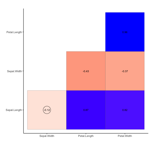
#' @examples
#' data(iris)
#' corrplot(iris[,1:4])
#'
#' @import ggplot2
#' @importFrom psych corr.test
#'
corrplot <- function(x, col = c("red", "white", "blue"), ...) {
corr <- psych::corr.test(x, ...)
corr_ci <- data.frame(raw.lower = corr$ci$lower, raw.r =
corr$ci$r,
raw.upper = corr$ci$upper, raw.p = corr$ci$p,
adj.lower = corr$ci.adj$lower.adj, adj.upper =
corr$ci.adj$upper.adj)
corr_ci$vars <- row.names(corr_ci)
corr_ci$conf_x <- unlist(sapply(1:(length(x)-1), function(i){
c(1:(length(x)-1))[i:(length(x)-1)]
})) + 1
rev_mat <- (length(x)-1):1
corr_ci$conf_y <- unlist(sapply(1:(length(x)-1), function(i){
rep(i, times = rev_mat[i])
}))
n_seq <- 2:length(x)
corr_ci$y_var <- unlist(sapply(1:(length(x)-1), function(i){
rep(row.names(corr[[1]])[i], rev_mat[i])
}))
corr_ci$x_var <- unlist(sapply(1:(length(x)-1), function(i){
row.names(corr[[1]])[n_seq[i]:length(x)]
}))
corr_ci$x_var <- factor(corr_ci$x_var, levels =
unique(corr_ci$x_var))
corr_ci$y_var <- factor(corr_ci$y_var, levels =
unique(corr_ci$y_var))
corr_ci$conf <- (corr_ci$raw.lower > 0) == (corr_ci$raw.upper
> 0)
corr_ci$raw.r <- round(corr_ci$raw.r, 2)
ggplot2::ggplot() +
ggplot2::geom_tile(data = corr_ci,
ggplot2::aes(x = x_var, y = y_var,
fill = raw.r), colour = "black") +
ggplot2::geom_text(data = corr_ci,
ggplot2::aes(x = x_var, y = y_var, label = raw.r),
size = 3) +
ggplot2::geom_point(data = corr_ci[corr_ci$conf == FALSE,],
ggplot2::aes(x = x_var, y = y_var),
fill = NA, colour = "black", shape = 21, size = 11) +
ggplot2::scale_fill_gradient2(name = "r",
low = col[1], mid = col[2], high = col[3]) +
ggplot2::theme_classic() +
ggplot2::labs(x = "", y = "") +
ggplot2::coord_equal() +
ggplot2::theme(legend.position = "none")
}
corrplot(iris[,1:4])
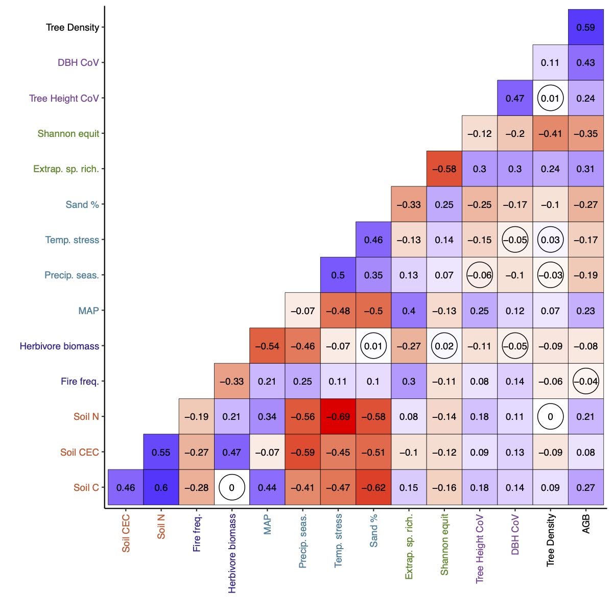
Here is the actual plot I made for the publication, which
additionally colours the axis text to group variables into latent
constructs: