TITLE: Constructing diversity profiles with Hill numbers
DATE: 2019-12-05
AUTHOR: John L. Godlee
====================================================================
Hill numbers represent a shared form of diversity indices. The
order (q) of a Hill number determines its sensitivity to rare vs.
abundant species, by modifying how the weighted mean of the species
proportional abundances is calculated. Common diversity indices are
special cases of Hill numbers:
q Diversity index
--- ---------------------------
0 Species richness
1 Exponential Shannon index
2 Inverse Simpsons index
Hill numbers show the "effective number of species". That is, the
number of equally abundant species needed to produce the observed
value of diversity. Compared to traditional diversity indices, the
relationship between Hill numbers and diversity is geometric. If
you double the number of species present with the same abundance,
the value of the Hill number will also double.
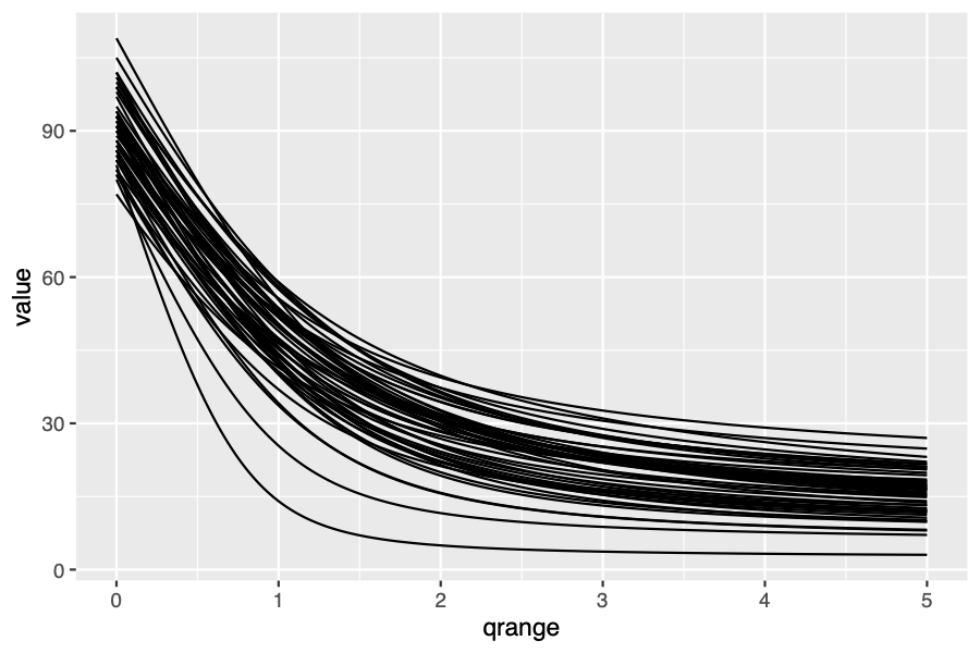
To investigate the contributions of rare and abundant species in a
community it is sometimes desirable to plot a diversity profile,
showing the value of diversity calculated along a continuum of the
order q. I wrote some R functions to do this easily.
# Load data
library(vegan)
data(BCI)
##' A species (columns) by site (rows) matrix of abundance
values
# Calculate diversity for any order q
qd <- function(data, q = 1){
# Convert to matrix
data <- drop(as.matrix(data))
# get relative abundance
data <- sweep(data, 1, apply(data, 1, sum), "/")
# Calculate hill numbers
if (q == 0) { # Richness
hill <- apply(data > 0, 1, sum, na.rm = TRUE)
} elseif (q==1) { # Shannon
data <- -data * log(data)
hill <- exp(apply(data, 1, sum, na.rm = TRUE))
} else { # Other Hill number
data <- data^q # p_i^q
hill <- (apply(data, 1, sum, na.rm = TRUE))^(1/(1 - q))
}
return(hill)
}
# Calculate hill numbers over range of q
qd_curve <- function(data, qmin = 0, qmax = 5) {
# Define range of q
qrange <- seq(from = qmin , to = qmax , by = 0.01)
# For each value of q, calculate hill numbers for each site
qdf <- sapply(qrange , function(x){
qd(data, x)
})
# Transpose to clean dataframe
qclean <- data.frame(cbind(qrange , t(qdf)))
names(qclean)[1] <- "qrange"
return(qclean)
}
qd_curve() returns a dataframe of sites (columns) by Hill number
order q (rows). This dataframe can then be used to plot a diversity
profile with a line for each site.
library(vegan)
library(ggplot2)
library(dplyr)
library(tidyr)
data(BCI)
qd_curve(BCI) %>%
gather("id", "value", -qrange) %>%
ggplot(., aes(x = qrange, y = value)) +
geom_line(aes(group = id))