TITLE: Analysing BibTeX files in R
DATE: 2019-09-12
AUTHOR: John L. Godlee
====================================================================
I have a master BibTeX file called lib.bib, which contains
bibliographic information on every paper I've read, which pairs
with a directory of those papers' .pdf files. I thought it would be
fun to see if there were patterns in my reading which I could find
by analysing lib.bib in R.
I have a bash script which extracts bibliographic information from
each BibTeX entry and stores it as a text file:
#!/bin/bash
# Extract year of publication
cat ~/google_drive/lib.bib | grep -E "year = [0-9]{4}" | grep
-oE "[0-9]{4}" > years.txt
# Extract all authors per paper, clean
cat ~/google_drive/lib.bib | grep -E "author = {" | sed 's/.*=
{\([^]]*\)},.*/\1/g' | sed 's/[^A-z \-]//g' | sed 's/\\//g' | sed
's/ and /,/g' > authors.txt
# Extract journal
cat ~/google_drive/lib.bib | grep -E "journal = {|publisher =
{|url = |institution = {|organization = {|school = {" | sed
's/.*{\([^]]*\)}.*/\1/g' > journals.txt
Rscript analysis.R
It makes three files, one containing the year of publication, one
containing the authors for each publication, and one containing the
publication name.
Extracting author names was the most difficult because names are
not always formatted the same, especially those names which contain
{van der} Putten for example, where the actual initial of the
surname is not v but P in the example above. One interesting trick
I found was using sed to extract text between the first occurrence
of one character, and the last occurrence of another character,
ignoring repeats of those characters. I used this to extract author
names between { } despite some authors having {van der} in their
surname:
sed 's/.*= {\([^]]*\)},.*/\1/g'
Then the bash script calls an R script:
# Packages
library(dplyr)
library(ggplot2)
library(igraph)
library(ggnetwork)
# Load data
years <- readLines("years.txt")
journals <- readLines("journals.txt")
authors <- readLines("authors.txt")
# Clean
authors_list <- strsplit(x = authors, split = ",")
papers <- data.frame(years = as.numeric(years), journals)
papers$authors <- authors_list
papers$num_authors <- sapply(authors_list, length)
papers$authors actually contains a list where each row is a vector
of author names for a paper
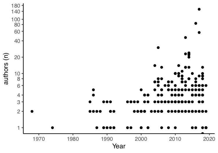
The first plot draws a correlation between year of publication and
number of authors:
# Plot correlation between year of publication and number of
authors
year_author_correl <- ggplot(papers, aes(x = years, y =
num_authors)) +
geom_point() +
theme_classic() +
labs(x = "Year", y = "authors (n)") +
scale_y_continuous(trans = 'log', breaks =
c(0,1,2,3,4,6,8,10,20,40,60,80,100,140,180))
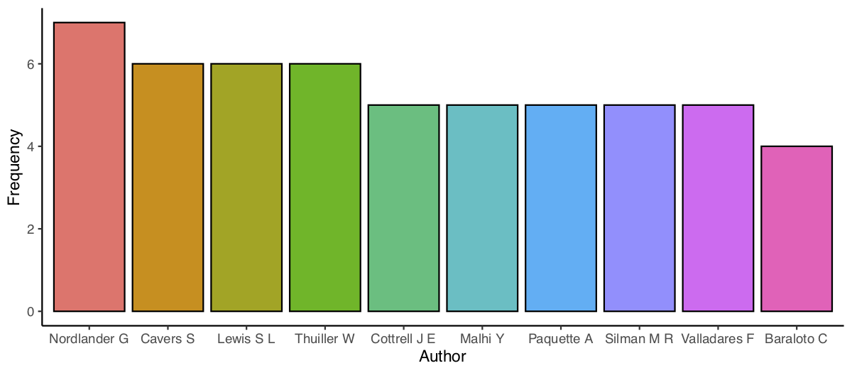
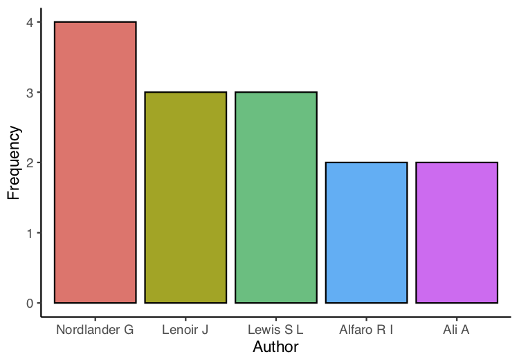
The next two plots are bar graphs of the frequency of the most
common authors (first and co-authors) and the most common first
authors:
## Get list of most common authors
author_all <- unlist(papers$authors)
## Get top ten authors
author_top_ten_df <- data.frame(sort(table(author_all),
decreasing = TRUE)[1:10])
names(author_top_ten_df) <- c("author", "freq")
## Plot
author_top_ten <- ggplot(author_top_ten_df, aes(x = author, y =
freq)) +
geom_bar(stat = "identity", aes(fill = author), colour =
"black") +
theme_classic() +
theme(legend.position = "none") +
labs(x = "Author", y = "Frequency")
## Get top first authors
author_common <- unlist(lapply(papers$authors, first))
author_common_df <- data.frame(sort(table(author_common),
decreasing = TRUE)[1:5])
names(author_common_df) <- c("author", "freq")
author_common_df_clean <- author_common_df %>%
filter(freq > 1)
## Plot
first_author_top <- ggplot(author_common_df_clean, aes(x =
author, y = freq)) +
geom_bar(stat = "identity", aes(fill = author), colour =
"black") +
theme_classic() +
theme(legend.position = "none") +
labs(x = "Author", y = "Frequency")
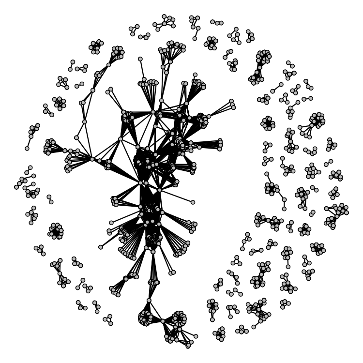
The final plot is a network graph of shared authorship. This isn't
perfect. What I would ideally like is to draw ellipses around
groups of authors on the same paper, to see whether groups of
authors tend to publish together multiple times, but I couldn't
figure out how to do it with an igraph object:
## Create edge list
authors_list_df <- list()
for(i in 1:length(papers$authors)){
authors_list_df[[i]] <- data.frame(author =
papers$authors[[i]])
authors_list_df[[i]]$paper_id <- rep(i, times =
length(papers$authors[[i]]))
}
authors_df <- bind_rows(authors_list_df)
authors_edge_df <- authors_df %>%
inner_join(., authors_df, by = "paper_id") %>%
filter(author.x != author.y) %>%
count(author.x, author.y, paper_id)
authors_vertex_meta <- authors_edge_df[,3]
authors_edge <- authors_edge_df[,1:2] %>%
graph_from_data_frame(., directed = FALSE)
authors_edge_fort <- fortify(authors_edge)
## Plot
author_network <- ggplot(authors_edge_fort) +
geom_edges(aes(x = x, y = y, xend = xend, yend = yend), size
= 0.5) +
geom_point(aes(x = x, y = y), colour = "black", fill =
"grey", shape = 21) +
theme_void()