TITLE: A guide about processing hemispherical photos
DATE: 2018-09-07
AUTHOR: John L. Godlee
====================================================================
I wrote a guide for some undergraduate students on a field course
about hemispherical photography and calculating forest canopy
traits. This is it. It's untested so far, so some parts may change
depending on how well the field course goes. The guide may get
updated, so the most up to date version can always be found here,
on Github.
[here, on Github]:
https://github.com/johngodlee/hemi_photo_guide
Part 1 - Taking hemispherical photos
A list of tips for taking good hemispherical photos:
- Take photos under a uniformly overcast sky, ideally before the
sun has risen too high in the sky, or just before sunset. I find in
the morning the photos are generally better and at high latitudes
you will have more time than in the tropics..
- Ensure that the camera is level and the lens is pointing
straight up. Use the spirit level on the camera hotshoe to do this.
- Adjust the tripod so that the top of the camera lens is 1 m
above the ground, or above any understorey vegetation, whichever is
higher.
- Turn the camera so the top of the camera body is facing north,
take a compass! This ensures that the top of the captured photo is
also facing north, which is necessary for calculating LAI..
- Make use of the articulated display on the camera to get a good
view of the photo before you take it.
- Set the camera:
- Manual shooting mode
- Manual focus
- Set the focus to infinity
- Exposure compensation = -0.7
- Capturing fine jpeg & RAW images at the same time
- The camera time and date is accurate (this is purely for
ease of matching photos to sites)
- Set the Aperture to 5
- Adjust the ISO and shutter speed so the photo is neutrally
exposed but the shutter speed is always over 1/60sec, otherwise you
will introduce camera shake when you press the button
- Take all photos in landscape dimensions, never portait.
- Make sure you all duck down below the camera when the image is
being taken!
- Make sure there is battery and you have the spare battery
- Make sure there is an SD card in the camera, and take a spare.
- Cover the lens with the lens cap between photos. PLEASE PLEASE
PLEASE!!!
Part 2 - Creating a black and white thresholded image
1. Open ImageJ
2. File -> Open, then select an image
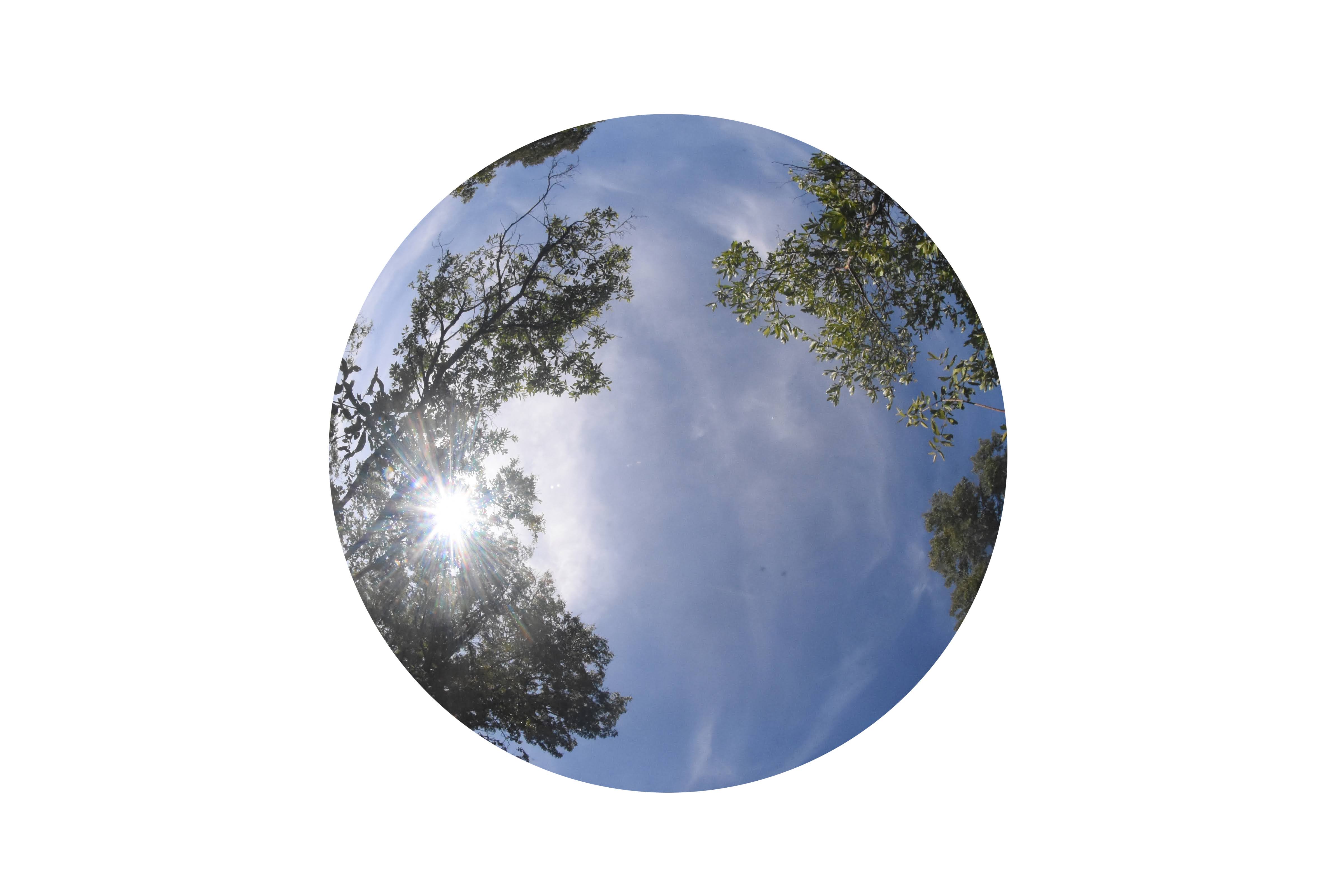
3. Visually inspect the image to see that there isn't massive
amounts of lens flare. If you have lots of lens flare, the photo
should be thrown out! This is what lens flare looks like:
4. Image -> Type -> 8-bit
5. Image -> Adjust -> Threshold, manually adjust the image so all
the branches are red and the sky is white, or as near as you can
get it.
6. Save the newly thresholded image as a jpeg in a folder called
img.
7. Rinse and repeat for all images.
The above process can be automated with a macro, but this assumes
that the images are all uniformly exposed.
This is the macro, saved as a .ijm file. This is untested so use at
your own risk:
// Automatically create a thresholded image for use in further
analysis. Change the values of setThreshold to achieve different
results.
// Partially tested
// Save as a Jpeg in the Batch macro dialog in ImageJ
run("8-bit");
run("Threshold...");
setThreshold(0, 146);
setOption("BlackBackground", false);
run("Convert to Mask");
Part 3 - Calculating Leaf Area Index
1. Open RStudio.
2. Open a new script (File -> New File -> R Script)
3. Save the script in a folder above the images folder:
4. Enter the following preamble into the R script:
# Set working directory to location of thresholded images
setwd("LOCATION_OF_ANALYSIS")
# Source the functions used to calculate stuff
source("hemiphot.R")
# Packages
library(jpeg)
5. Add white_image.jpg to the same folder where the thresholded
images are found
6. Read in all the thresholded images and create an empty data
frame which will later be filled with canopy trait statistics like
LAI and canopy openness.
# List all images in the directory
all_images <- list.files("img/", pattern = ".JPG")
# How many images
img_length = length(all_images)
# Create empty dataframe, 6x7 and fill it with zeroes
all_data = data.frame(matrix(data = 0, nrow = img_length, ncol
= 7))
names(all_data) = c("File", "CanOpen", "LAI", "DirectAbove",
"DiffAbove", "DirectBelow", "DiffBelow")
# Fill first column with image names
all_data[,1] = all_images
7. Read in the reference image (white_img.jpg) as a matrix of
pixel values:
white_img <- readJPEG("img/white_image.jpg", native = F)
8. Set some parameters for the location the photos are being
taken. Approximate location (0.1 degrees latitude) is good enough
for our purposes. Note that the values below are for somewhere in
Africa and should be changed:
location.latitude = -15
location.altitude = 200
location.day = 30
location.days = seq(15,360,30) # roughly each mid of
the 12 months
9. Set some parameters for the images, cropping them to a circle
and setting the threshold. These parameters are ones I have used on
this camera, so don't need to be changed:
## Image parameters
### Drawing circles and identifying the image centre point
hemi_dim <- dim(white_img)
radius <- max(rowSums(white_img[,,1] > 0.4) / 2)
### determine using a single image and fill in here for batch
processing
location.cx = (hemi_dim[2] / 2) # x
coordinate of center of image
location.cy = (hemi_dim[1] / 2) # y
coordinate of center image
location.cr = radius # radius of circle
location.threshold = 0.42 # Must get this to match all
images, or maybe could use a lookup table / dictionary? Does R
have dictionaries?
10. Set some atmospheric parameters. I've loosely estimated these
for this location, but by no means is it scientific. I would not
have much confidence in the statistics generated using these
parameters, namely DirectAbove, DiffAbove, DirectBelow and
DiffBelow.
# atmospheric parameters
## Atmospheric transmissivity - Normally set at 0.6, but can
vary between 0.4-0.6 in the tropics
location.tau = 0.6
## Amount of direct light that is used as diffuse light in the
Uniform Ovecast Sky (UOC)
location.uoc = 0.15
11. Run a big for loop to calculate the statistics for each photo
for(i in 1:img_length){
## read file
image <- readJPEG(paste("test_img/", all_images[i], sep =
""), native = F)
## conver to Hemi image
image <- Image2Hemiphot(image)
## set cirlce parameters
image <- SetCircle(image, cx = location.cx, cy =
location.cy, cr = location.cr)
## select blue channel
image <- SelectRGB(image, "B")
#threshold
image <- ThresholdImage(im = image, th =
location.threshold, draw.image = F)
# canopy openness
gap.fractions <- CalcGapFractions(image)
all_data[i,2] = CalcOpenness(fractions = gap.fractions)
## calculate LAI according to Licor's LAI Analyzer
all_data[i,3] = CalcLAI(fractions = gap.fractions)
## Photosynthetic Photon Flux Density (PPDF, umol m-1 s-1) P
rad <- CalcPAR.Day(im = image,
lat = location.latitude, d = location.days,
tau = location.tau, uoc = location.uoc,
draw.tracks = F,
full.day = F)
all_data[i,4] = rad[1]
all_data[i,5] = rad[2]
all_data[i,6] = rad[3]
all_data[i,7] = rad[4]
}
12. Finally, look at the output, which is stored in all_data
all_data
The hemiphot.R source file comes from here.
[here]:
https://github.com/naturalis/Hemiphot