TITLE: Using R to locate spatial data points inside map polygons
DATE: 2017-09-27
AUTHOR: John L. Godlee
====================================================================
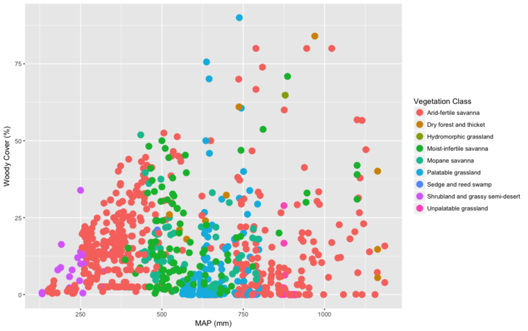
I was looking into a paper called "Determinants of woody cover in
African savannas" by Sankaran et al. (2005). The paper looks at the
large scale environmental factors that affect percentage woodland
cover in African savanna landscapes. One figure in particular that
got me interested was this one:

I haven't fully worked out the implications of this figure yet, but
what stands out to me the most is that many plots in high rainfall
areas with low woody cover are classed as 'arid fertile savanna' by
White's veg. classification. Secondly moist infertile savanna seems
to straddle the saturation point of the MAP limited woody cover.
It shows that savannas with Mean Annual Precipitation values less
than ~650 mm have their upper woody cover potential limited by
precipitation, but above that threshold an increase in MAP doesn't
increase the maximum potential woody cover. It also shows that lots
of sites have woody cover below their MAP limited maximum, pointing
to lots of other environmental factors, like fire, herbivory, soil
characteristics.
Looking into this graph more, I wanted to see whether there was any
biogeographic patterns that could be drawn from the data. Were all
the sites with particularly low actual woody cover from a
particular woodland cover biome, for example.
To do this I compared the data from Sankaran et al. (2005), which
is publicly available as supplementary information, to White's
seminal vegetation classification map of 1983, which I accessed as
as shapefiles from here.
I did this analysis in R, so all the code below is for R.
You can find the code and data that I used by cloning this github
repo.
First, I loaded the packages and the data:
# Set working directory to the location of the source file ----
setwd(dirname(rstudioapi::getActiveDocumentContext()$path))
# Packages ----
library(ggplot2)
library(dplyr)
library(rgeos)
library(rgdal)
# Import data ----
## sankaran data
cover <- read.csv("data/sankaran_2005_data.csv")
str(cover)
## white 1983 veg data
white_veg <- readOGR(dsn="data/whitesveg",
layer="Whites vegetation")
## Country outline
countries <- readOGR(dsn="data/africa",
layer="Africa")
First I can have a go at plotting White's map:
# Plot White's veg map data ----
## Fortify country outline for ggplot
countries@data
countries_fort <- fortify(countries, region = "COUNTRY")
## Exploring whiteveg
white_veg@data
white_veg@polygons[[1]]
white_veg@proj4string
white_veg@bbox
white_veg@plotOrder
## Fortify white shape file for ggplot2
white_veg_fort <- fortify(white_veg, region = "DESCRIPTIO")
names(white_veg_fort)
length(unique(white_veg_fort$id))
## Create colour palette for ggplot2
palette_veg_type_19 <-
c("#FF4A46","#008941","#006FA6","#A30059","#FFDBE5",
"#7A4900","#0000A6","#63FFAC","#B79762","#004D43",
"#8FB0FF","#997D87","#5A0007","#809693","#FEFFE6",
"#1B4400","#4FC601","#3B5DFF","#4A3B53")
## ggplot
ggplot() +
geom_polygon(aes(x = long, y = lat, group = group, fill =
id),
data = white_veg_fort) +
geom_polygon(aes(x = long, y = lat, group = group, fill =
NA),
colour = "black",
data = countries_fort) +
theme_classic() +
scale_fill_manual(values = palette_veg_type_19) +
labs(fill = "Biome") +
xlab("Longitude") +
ylab("Latitude") +
coord_map()
Then I had to convert the data from Sankaran et al. into a
SpatialPoints object so I can use it in future analyses.
# Create a data frame with only the latitude and longitude data
cover_coords <- cover %>%
select(lon_dec_deg, lat_dec_deg) # Important for later on
to have lon then lat as columns
# Convert to SpatialPoints object
cover_spoints <-
SpatialPoints(cover_coords,proj4string=CRS(proj4string(white_veg)))
The bit of this project that took me some time to work out was how
to compute whether a data point from Sankaran et al. fell into a
polygon of a certain type in White's map. I ended up using over()
from the sp package. Then I can add that data back into the
original Sankaran dataset
# Add vegetation class column by referencing White map
cover_veg_class <- cover %>%
mutate(veg_class = over(cover_spoints,
white_veg)$DESCRIPTIO)
Finally, I can use cover_veg_class to create a ggplot of MAP vs
woody cover, with the points coloured according to which of White's
vegetation classes the point is in:
# Plot with vegetation classification from White et al. 1983
----
veg_class_plot <- ggplot(cover_veg_class, aes(x = map_mm,
y = woody_cover_per,
colour = veg_class)) +
geom_point(size = 4) +
guides(colour=guide_legend(title="Vegetation Class")) +
xlab("MAP (mm)") +
ylab("Woody Cover (%)")