TITLE: Mapping The Vegetation and Climate of Africa in R
DATE: 2017-09-05
AUTHOR: John L. Godlee
====================================================================
As I'll soon be embarking on my PhD research into biodiversity and
woodland productivity in Southern Africa, I thought I should get a
better idea of how the vegatation differs across the continent.
I normally try to use R instead of point and click GIS packages
like ArcMap or QGIS, so all the code here is to be used in an R
session.
The packages I used are:
library(maps)
library(rgdal)
library(ggplot2)
library(ggmap)
First I needed a base map of Africa, ideally with countries on,
which I found here.
[which I found here]:
http://maplibrary.org/library/stacks/Africa/index.htm
# Import shapefile of country borders ----
countries <- readOGR(dsn="africa",
layer="Africa")
countries@data
countries_fort <- fortify(countries, region = "COUNTRY")
# Plot country borders ----
ggplot() +
geom_polygon(aes(x = long, y = lat, group = group, fill =
NA),
colour = "black",
data = countries_fort) +
theme_classic() +
scale_fill_manual(values = palette_veg_type_19) +
labs(fill = "Biome") +
xlab("Longitude") +
ylab("Latitude") +
coord_map()
To investigate vegetation types I tracked down a shapefile version
of White's 1983 Vegetation Map. The map is the result of 15 years
of work by UNESCO and AEFTET and was created by first compiling
many existing maps, then cross-checking with extensive fieldwork
and consultation with local experts.
[shapefile version of White's 1983 Vegetation Map]:
http://omap.africanmarineatlas.org/BIOSPHERE/pages/3_terrestrial%20v
egetation.htm
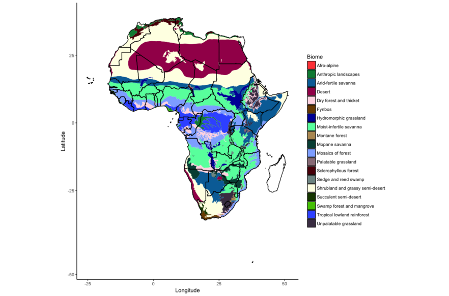
To create the map above I used the ggplot2 and rgdal packages:
# Read shapefile ----
white_veg <- readOGR(dsn="whitesveg",
layer="Whites vegetation")
# Explore shapefile
white_veg@data
white_veg@bbox
white_veg@proj4string
# Fortify shapefile for use in ggplot2 ----
white_veg_fort <- fortify(white_veg, region = "DESCRIPTIO")
names(white_veg_fort)
length(unique(white_veg_fort$id))
# Create colour palette for ggplot2 ----
palette_veg_type_19 <-
c("#FF4A46","#008941","#006FA6","#A30059","#FFDBE5",
"#7A4900","#0000A6","#63FFAC","#B79762","#004D43",
"#8FB0FF","#997D87","#5A0007","#809693","#FEFFE6",
"#1B4400","#4FC601","#3B5DFF","#4A3B53")
# ggplot Africa with vegetation ----
ggplot() +
geom_polygon(aes(x = long, y = lat, group = group, fill =
id),
data = white_veg_fort) +
geom_polygon(aes(x = long, y = lat, group = group, fill =
NA),
colour = "black",
data = countries_fort) +
theme_classic() +
scale_fill_manual(values = palette_veg_type_19) +
labs(fill = "Biome") +
xlab("Longitude") +
ylab("Latitude") +
coord_map()
To look specifically at Southern Africa I had to use some trial and
error to get the x and y limits right in the ggplot() call:
# ggplot Southern Africa ----
ggplot() +
geom_polygon(aes(x = long, y = lat, group = group, fill = id),
data = white_veg_fort) +
geom_polygon(aes(x = long, y = lat, group = group, fill = NA),
colour = "black",
data = countries_fort) +
theme_classic() +
scale_fill_manual(values = palette_veg_type_19) +
labs(fill = "Biome") +
xlab("Longitude") +
ylab("Latitude") +
coord_map(xlim = c(10, 40), ylim = c(-35, -10))
The steps once again for anyone interested in a mapping workflow in
R:
1. Import shapefile with readOGR()
2. Explore shapefile
3. "Fortify" shapefile for use in ggplot()
4. Plot using ggplot()
I also wrote a tutorial for the Coding Club group I'm involved with
on using R as a GIS